
[Trouble Shooting] Visualization with Matplotlib & Seaborn
데이터의 종류에는 대표적으로 수치형(numerical)과 범주형(categorical)이 있다. 수치형은 길이, 무게, 온도와 같은 연속형(continuous)과 주사위 눈금, 사람 수 등의 이산형(discrete) 데이터가 있다. 범주형은 혈액형이나 종교 같은 명목형(norminal)과 학년, 벌점, 등급 등 순서형(ordinal) 데이터로 구분할 수 있다.
또한 정형데이터, 시계열 데이터, 지리데이터, 관계형(네트워크) 데이터, 계층적 데이터, 다양한 비정형 데이터 등 수 많은 데이터셋이 존재한다. 데이터 시각화는 이러한 데이터들을 이해하기 쉽고 가치 있는 정보를 얻을 수 있도록 만들 수 있고, 의사결정에도 큰 도움이 될 수 있다. 이 포스트에서는 목적에 따른 시각화 기법을 잘 선택히여 활용할 수 있도록, 그리고 상대방이 효과적으로 수용할 수 있는 시각화 결과를 만들어낼 수 있도록 정리해보고자 한다.
시각화 이해
- 시각화는 점, 선, 면에서부터 시작한다.
- 아래에서 다룰
Matplotlib이나Seaborn같은 시각화 툴들은 점, 선, 면을 다양하게 변경할 수 있는 기능을 제공한다. - 시각화를 할 때 중요한 것은 화려하다고 좋은 것이 아니다. 원하는 목적에 맞는 시각화여야 하며 Pre-attentive 에 주의해야 한다.
- 이는 주의를 주지 않아도 인지하게 되는 요소로, 시각적으로 다양한 Pre-attentive 속성이 존재한다.
- 방향, 길이, 너비, 크기, 모양, 대비, 강조, 위치 등 다양한 요소들이 존재하며, 여러 개를 동시에 사용하면 오히려 인지하기 어렵고 적절하게 사용해야 한다.
시각화 분류
- 시각화를 분류할 때는 아래와 같다.
- 시간 시각화
- 시간 흐름에 따른 변화를 표현한다. 주로 x 축을 시간, y 축을 값으로 표현하며, 막대 그래프, 산점도, 선 그래프, 계단 그래프, 영역 차트 등을 이용한다.
- 막대 그래프(Bar Plot)는 범주형 변수의 빈도를 활용한다. 여기서 더 나아가 Stacked Bar Plot 이나 Overlapped Bar Plot 등을 사용할 수 있다. 또한 하나의 변수가 여러 unique 값을 가질 때 이를 표현할 수 있는데 이 때 Count plot 도 유용하다.
- 관계 시각화
- 다변량 데이터에 대하여 변수 간의 연관성 및 패턴을 색상, 농도 등을 사용하여 표현 및 분석한다. 산점도, 산점도 행렬, 버블 차트, 히트맵 등을 이용한다.
- 산점도(Scatter Plot)의 경우 두 수치형 변수의 상관관계를 알아볼 수 있고, 이 때 범주별로 색상, 모양, 크기 등을 변경하여 더 많은 정보를 담을 수도 있다.
- 산점도 행렬의 경우 여러 수치형 변수의 상관관계를 알아보는데, seaborn 의 Pair plot 으로 그려볼 수 있다.
- 버블 차트(Bubble Chart)의 경우 산점도와 비슷하지만 데이터의 크기, 범주를 버블의 크기, 색상으로 나타낸다.
- 비교 시각화
- 다변량 데이터에 대하여 유사 또는 차이에 대해 점, 선, 막대, 색상 등을 사용하여 표현한다. 평행 차트, 히트맵, 스타 차트, 플로팅 바 차트, 체르노프 페이스, 다차원 척도법(MDS) 등이 있다.
- 평행 차트(Parallel Chart)는 입력 feature 의 개수 만큼 Y 축을 만들고 동일한 행에 있는 값을 선으로 연결하여 표시한다. 즉 하나의 데이터 포인트를 한 눈에 볼 수 있다.
- 스타 차트(Star Chart)의 경우, Spider, Rader Chart 라고도 부른다. 이는 측정 목표에 대한 평가 항목이 다수일 때 사용한다. 변수의 수 만큼 축을 그리고 각 축에 측정값을 표시하여 항목 간 비율 및 균형/경향을 알 수 있다.
- 히트맵(Heat Map)의 경우 두 개 범주형 변수의 관계/비교 시각화에 사용한다. 색 및 농도를 사용하여 값의 크기를 표시한다.
- 플로팅 바(Floating Bar)의 경우 축에 연결되지 않고 최소/최대 값 사이에 하나 또는 여러 막대가 떠 있는 차트다. 온도, 주가, 혈압 등의 범위 표시에 유용하다.
- 공간 시각화
- 지도를 활용하여 데이터를 표현한다. 코로플레스(Choropleth Map), 카토그램(Cartogram), 버블 플롯맵 등이 있다.
- 코로플레스 지도는 데이터 값의 크기에 따라 한 색상의 명도를 몇 단계로 나누어 지역 별 데이터를 표시한다.
- 카토그램은 데이터 값의 변화에 따라 지도의 면적이 왜곡되는 지도다. 데이터 값이 큰 지역의 면적이 더 크게 표시된다.
- 버블 플롯맵은 버블 차트에 위도, 경도 정보를 적용한 것이다.
- 구성 시각화
- 범주형 데이터의 구성(composition)을 크기로 표현한다. 파이 차트, 도넛 차트, 트리 맵 차트 등이 있다.
- 파이 차트(Pie Chart)의 경우 원의 조각을 사용하여 범주형 데이터의 범주별 기여도를 표시하는데 사용한다.
- 도넛 차트(Donut Chart)의 경우 파이 차트 중앙에 구멍을 넣어 표현한 것으로, 표현 내용은 파이 차트와 동일하지만 여러 범주 데이터에 대해 선버스트 차트(Sunburst Chart)를 사용할 수 있다.
- 트리 맵 차트(Tree Map Chart)는 계층 구조를 나타내며 사각형의 크기 또는 면적을 사용하여 구성/비율을 나타낸다.
- 분포 시각화
- 연속형 데이터의 분포를 시각적으로 표현한다. 1 개 변수일 때는 히스토그램과 박스 플롯, 2 개 변수일 때는 산점도를 사용한다.
- 히스토그램(histogram)에서 막대 높이는 빈도를 나타내며 폭은 의미가 없다. 가로/세로축 모두 연속적이며 많은 데이터를 가지고 있는 경우에 정확한 관계 파악을 용이하게 해준다.
- 박스 플롯(Box Plot)의 경우 수치형 변수의 분포 및 이상치를 확인하는데 사용된다.
- 시간 시각화
- 이처럼 시각화 방법에는 매우 다양한 기법들이 존재한다. 무작정 암기하기 보다 아래에 시각화에 대한 예시들을 모아둔 Matplotlib 과 Seaborn 공식문서 gallery 를 충분히 활용하고 눈에 담으며 적재적소에 떠올려 활용해보도록 하자.
Matplotlib
Matplotlib은 Python 에서 사용할 수 있는 시각화 라이브러리다. 현재 사용되고 있는 다양한 데이터 분석 및 머신러닝/딥러닝은 Python 에서 이뤄지고 있는 만큼, 가장 많이 사용된다.- 또한
numpy와scipy를 베이스로 하여Scikit-Learn,PyTorch,Tensorflow,Pandas와 같은 다양한 라이브러리와 호환성이 좋다. - 다양한 시각화 방법론을 제공한다.
- 그 외에도
Seaborn,Plotly,Bokeh,Altair등의 시각화 라이브러리가 존재하지만,Matplotlib이 범용성이 제일 넓고, base 가 되는 라이브러리이다. - 일반적으로
Matplotlib에서 가장 많이 사용하는pyplot모듈을 import 한다.
import matplotlib.pyplot as plt
plt.style.use("default")

plt.style.available
- 이 때
style.use()를 주어 시각화의 스타일을 조정할 수 있다.plt.style.available로 사용 가능한 스타일을 확인할 수 있다."defualt"로 하면 일반적으로 보는 흰 배경이 나온다. - matplotlib 에서 그리는 시각화는 Figure 라는 큰 틀에 Ax 라는 서브플롯을 추가해서 만든다.
- 다만 Figure 는 큰 틀이기 때문에 서브플롯을 최소 1 개 이상 추가해야 하고, 추가하는 다양한 방법이 있다.
fig = plt.figure(figsize=(16, 7))
ax1 = fig.add_subplot(211) # ax1 = fig.add_subplot(2, 1, 1)
ax2 = fig.add_subplot(212) # ax2 = fig.add_subplot(2, 1, 2)

plt.show()
plt.figure()안에figsize=()를 주게 되면 결과의 크기를 조절할 수 있다.- Ax 는
fig.add_subplot으로 Figure 안에 추가하게 되며, 인자로 위치를 지정해줄 수 있다.- 위 예제에서
211은 Figure 는(2, 1)의 크기를 가지며 그 중 첫번째에 위치하라는 것이다.
- 위 예제에서
-
plt.show()를 하지 않아도 시각화 결과가 보이지만,[<matplotlib.lines.Line2D at 0x10caa0130>]와 같은 출력이 나오게 된다.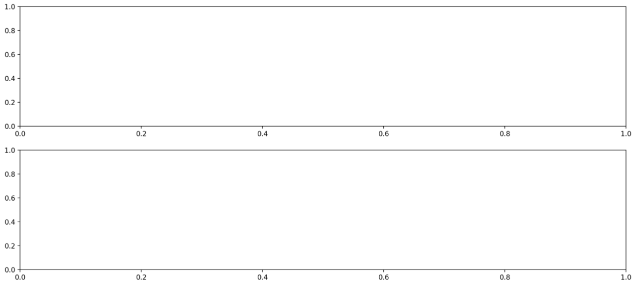
- 서브플롯을 추가하는 또 다른 방법은 아래와 같다.
.add_subplot()은 Ax 에 추가하지만,plt.subplots()로 서브플롯을 가진 Figure 를 그릴 수 있다.
fig, axes = plt.subplots(1, 2, figsize=(12, 7))

plt.show()
-
이 경우에 Ax 에 접근할 때는
axes[0]처럼 indexing 하는 식으로 접근한다.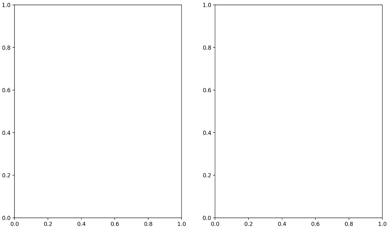
-
이제 단순하게
.plot()을 하면 선그래프를 그리게 된다. 주의할 점은 Ax 가 정의되면 그 밑에 그려진 plot 이 해당 Ax 에 들어가게 된다. 즉 순차적으로 Ax 에 plot 이 들어간다는 것이다.
fig = plt.figure()

x1 = [1, 2, 3]
x2 = [3, 2, 1]

ax1 = fig.add_subplot(211)
plt.plot(x1) # ax1 에 그리기. ax2 정의 이후에 나오면 ax2 에 그려진다.
ax2 = fig.add_subplot(212)
plt.plot(x2) # ax2 에 그리기
plt.show()
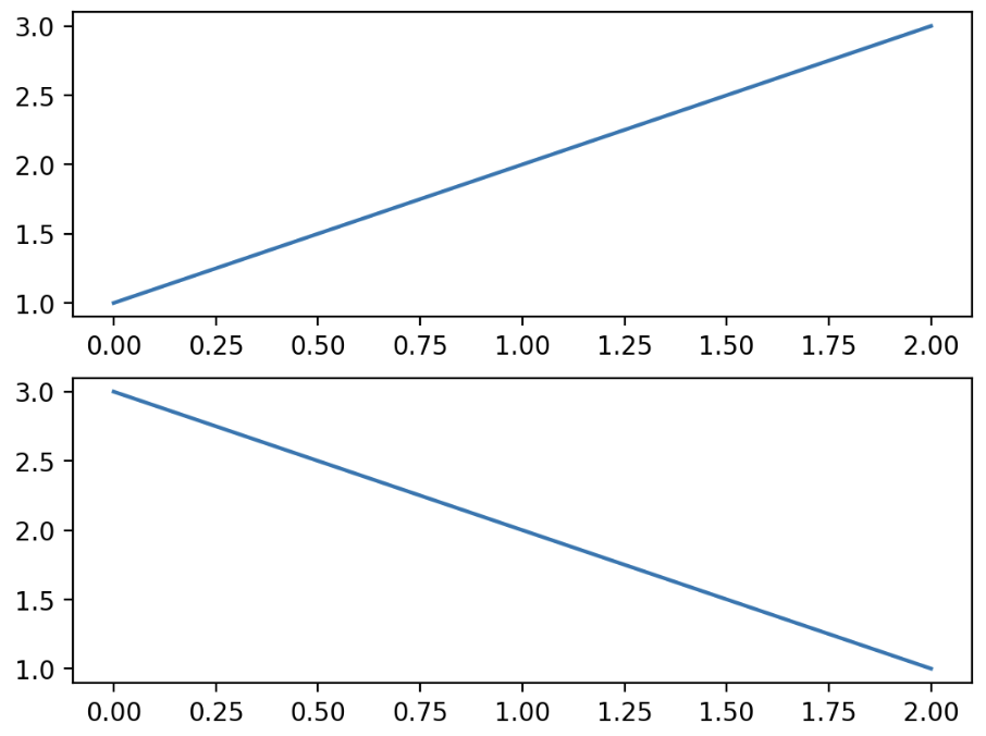
- 이 때 Ax 에 바로 그려줄 수도 있다. 아래 예제를 보자.
fig = plt.figure()

x1 = [1, 2, 3]
x2 = [3, 2, 1]

ax1 = fig.add_subplot(211)
ax2 = fig.add_subplot(212)

ax1.plot(x1) # ax1 에다가 그려달라고 명시
ax2.plot(x2)
plt.show()
-
결과는 아래와 같다.
-
또한 하나의 Ax 에는 다양한 그래프를 동시에 그릴 수 있다. 이 때 자동으로 색이 구분된다.
fig = plt.figure()
ax = fig.add_subplot()

ax.plot([1, 1, 1]) # 파랑
ax.plot([1, 2, 3]) # 주황
ax.plot([3, 3, 3]) # 초록

plt.show()
- 그러나 다른 종류의 그래프는 색 구분이 되지 않는다. 따라서 색을 직접 명시해주면 좋다. 색은
colorargument 로 전달한다.
fig = plt.figure()
ax1 = fig.add_subplot(121)
ax2 = fig.add_subplot(122)

ax1.plot([1, 2, 3], [1, 2, 3])
ax1.bar([1, 2, 3], [1, 2, 3])

ax2.plot([1, 2, 3], [1, 2, 3], color='r')
ax2.bar([1, 2, 3],[1, 2, 3], color='#123456')

plt.show()
- 위 예제처럼 색을 전달하는 방법은 한 글자로 주거나, hex code 로 주거나, color name 을 주면 된다.
- 한 글자로 정하는 색상은 원색 계열이 많고
'r', 'g', 'b', 'k'등이 있다. - hex code 는
#000000으로 표기하며 숫자 중 앞에서부터 두 개는 R, 그 다음 두 개는 G, 마지막 두 개는 B 를 뜻한다. 즉 16진수로 표현된다. -
color name 은 css 에서 사용하는 색들의 이름이다. 예를 들어
forestgreen등이 있다.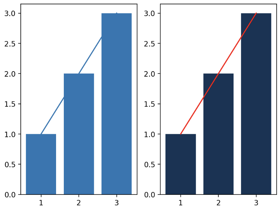
- 한 글자로 정하는 색상은 원색 계열이 많고
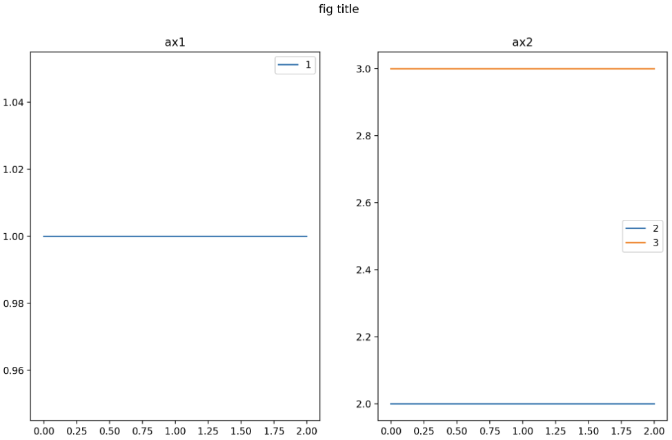
- 또한 시각화에서 정보를 추가하기 위해 텍스트를 사용할 수도 있다.
- 먼저
label을 줄 수 있다. 해당 label 정보는 범례(legend)가 추가되어야 보인다. - 그리고
.set_title()로 제목을 추가할 수 있다. 이는 Ax 에 주게 되면 해당 서브플롯의 제목을 의미하며, Figure 에는.suptitle()로 제목을 줄 수 있다. super title 을 의미한다.
fig = plt.figure(figsize=(12, 7))
ax1 = fig.add_subplot(1,2,1)
ax2 = fig.add_subplot(1,2,2)

ax1.set_title('ax1')
ax2.set_title('ax2')

ax1.plot([1, 1, 1], label='1')
ax2.plot([2, 2, 2], label='2')
ax2.plot([3, 3, 3], label='3')

fig.suptitle('fig title')
ax1.legend()
ax2.legend()
plt.show()
- 알아두면 좋은 것은 Ax 에서 특정 데이터를 변경하는 경우에 사용할 수 있는
.set_{}()형태의 메서드가 많다는 것이다. - 위
.set_title()처럼.set으로 세팅하는 정보들은, 반대로 해당 정보를 받아오는.get_{}()형태의 메서드로 확인할 수 있다.
print(len([method for method in dir(ax) if 'set_' in method]),
      len([method for method in dir(ax) if 'get_' in method]))
# 68, 88

print(ax1.get_title())  # ax1
- 추가적으로
ticks와ticklabels로 축에 대한 정보를 추가할 수 있다.
fig = plt.figure()
ax1 = fig.add_subplot(121)
ax2 = fig.add_subplot(122)

ax1.plot([1, 1, 1], label='1')
ax1.plot([2, 2, 2], label='2')
ax1.plot([3, 3, 3], label='3')

ax2.plot([1, 1, 1], label='1')
ax2.plot([2, 2, 2], label='2')
ax2.plot([3, 3, 3], label='3')

ax1.set_title('Basic Plot 1')
ax2.set_title('Basic Plot 2')

ax2.set_xticks([0, 1, 2, 3, 4])
ax2.set_xticklabels(['zero', 'one', 'two', 'three', 'four'])

ax1.legend()
ax2.legend()

plt.show()
-
set_xticks()축에 적히는 수를 정할 수 있다.set_xticklabels()는 축에 적히는 텍스트를 수정한다.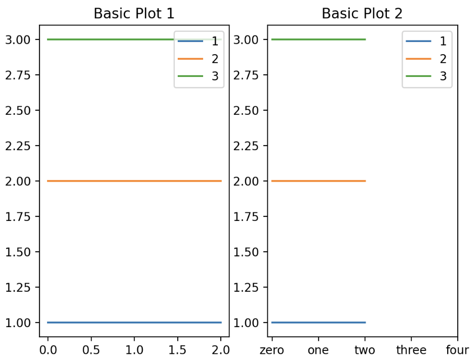
-
마지막으로 시각화 plot 에 텍스트를 추가하는 메서드는
.text()와.annotate()가 있다.
fig = plt.figure()
ax1 = fig.add_subplot(121)
ax2 = fig.add_subplot(122)

ax1.plot([1, 1, 1], label='1')
ax1.plot([2, 2, 2], label='2')
ax1.plot([3, 3, 3], label='3')

ax2.plot([1, 1, 1], label='1')
ax2.plot([2, 2, 2], label='2')
ax2.plot([3, 3, 3], label='3')

ax1.set_title('Basic Plot 1')
ax2.set_title('Basic Plot 2')

ax2.set_xticks([0, 1, 2])
ax2.set_xticklabels(['zero', 'one', 'two'])

ax1.text(x=1, y=2, s='This is Text', fontsize=15) # text
ax2.annotate(text='This is Annotate', xy=(1, 2), fontsize=10) # annotate

ax1.legend()
ax2.legend()

plt.show()
-
.text()와.annotate()는 용도가 살짝 다르다..text()는 원하는 위치에 적어서 정보를 나타는데 자주 쓰이고,.annotate()는 plot 위에 원하는 위치를 건네주면 해당 포인트에 텍스트를 지정해줄 수 있다.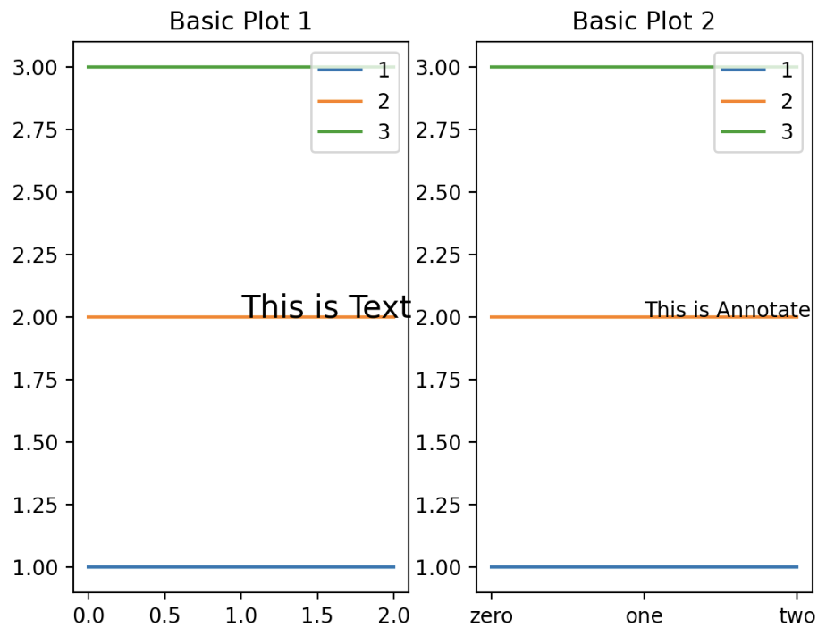
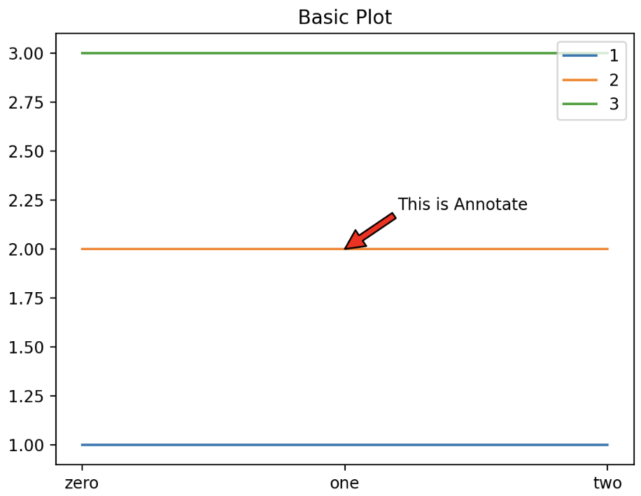
-
또한
.annotate()는 화살표 등을 추가할 수 있는 장점이 있다.
fig = plt.figure()
ax = fig.add_subplot(111)
ax.plot([1, 1, 1], label='1')
ax.plot([2, 2, 2], label='2')
ax.plot([3, 3, 3], label='3')


ax.set_title('Basic Plot')
ax.set_xticks([0, 1, 2])
ax.set_xticklabels(['zero', 'one', 'two'])

ax.annotate(text='This is Annotate', xy=(1, 2),
           xytext=(1.2, 2.2),
           arrowprops=dict(facecolor='red'),
           )

ax.legend()
plt.show()
barplot
- Bar plot 이란 직사각형 막대를 사용하여 데이터의 값을 표현하는 차트/그래프다. 막대 그래프, bar chart, bar graph 등의 이름으로 사용된다.
- Bar plot 은 범주(category)에 따른 수치 값을 비교하기에 적합한 방법이다. 개별 비교, 그룹 비교 모두 적합하다.
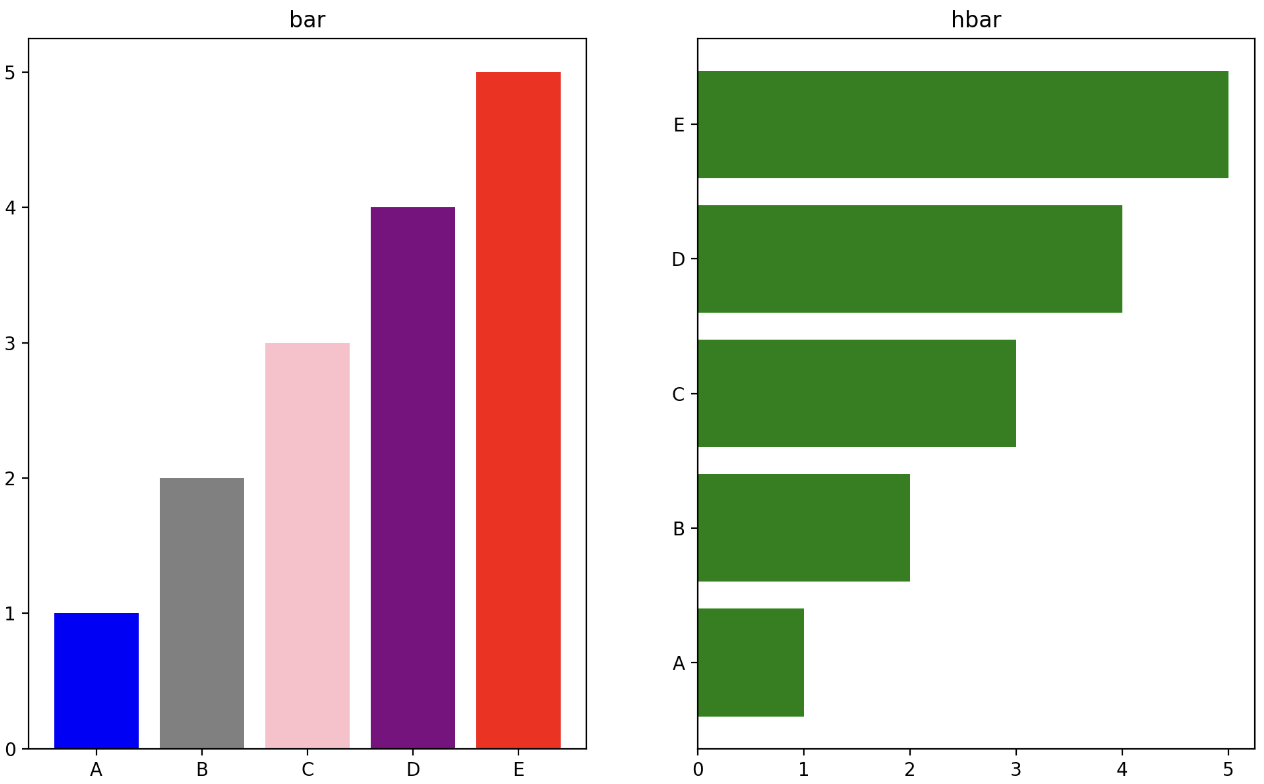
bar()는 기본적인 bar plot 이고,barh()은 수평(horizontal) 방향의 bar plot 이다.- 그리고 막대 그래프의 색은 개별로 변경할 수도 있고, 전체로 변경할 수도 있다. 개별로 색을 변경할 때는 list 로 전달하고, 막대 개수와 색의 개수가 같아야 한다.
fig, axes = plt.subplots(1, 2, figsize=(12, 7))

x = list('ABCDE')
y = np.array([1, 2, 3, 4, 5])

clist = ['blue', 'gray', 'pink', 'purple', 'red']
color = 'green'
axes[0].bar(x, y, color=clist)  # color list
axes[1].barh(x, y, color=color) # 전체 컬러

axes[0].set_title('bar')
axes[1].set_title('hbar')

plt.show()
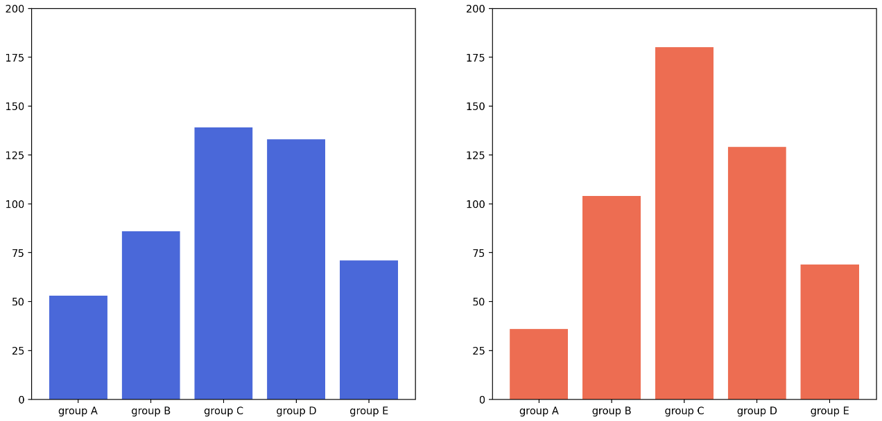
- 이제 데이터프레임에 plot 들을 적용해보자. 데이터는 캐글의 Student Exam Score 데이터를 이용한다.
ax.set_ylim()을 통해 y 축의 범위를 개별적으로 조정할 수 있다. 즉 scale 을 맞춰주는 것인데, 이를 통해 좀 더 객관적으로 비교가 가능하다.
fig, axes = plt.subplots(1, 2, figsize=(15, 7))

group = student.groupby('gender')['race/ethnicity'].value_counts().sort_index()

axes[0].bar(group['male'].index, group['male'], color='royalblue')
axes[1].bar(group['female'].index, group['female'], color='tomato')

for ax in axes:
    ax.set_ylim(0, 200)

plt.show()
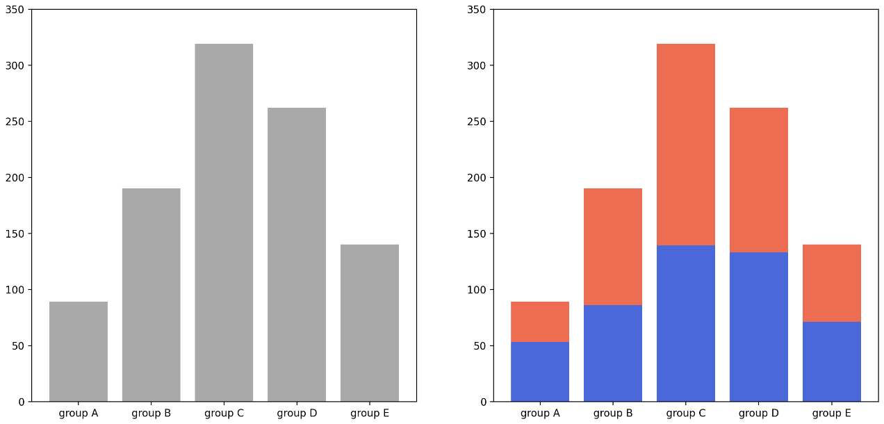
- 이 때 그룹 간 비교를 한눈에 보기 위하여 Stacked bar plot 을 사용할 수 있다.
bottomargument 를 이용하면 된다.
fig, axes = plt.subplots(1, 2, figsize=(15, 7))

group_cnt = student['race/ethnicity'].value_counts().sort_index()
axes[0].bar(group_cnt.index, group_cnt, color='darkgray') # 전체
axes[1].bar(group['male'].index, group['male'], color='royalblue')
axes[1].bar(group['female'].index, group['female'], bottom=group['male'], color='tomato')

for ax in axes:
    ax.set_ylim(0, 350)

plt.show()
- 이를
barh에서 사용하면leftargument 를 이용하면 된다. 이 때 각 그룹의 비율을 나타낼 수도 있다. 아래 예제를 보자.
fig, ax = plt.subplots(1, 1, figsize=(12, 7))

group = group.sort_index(ascending=False) # 역순 정렬
total=group['male']+group['female'] # 각 그룹별 합

ax.barh(group['male'].index, group['male']/total, color='royalblue')
ax.barh(group['female'].index, group['female']/total, left=group['male']/total, color='tomato')

# 그래프 내 4개 축을 제거하면 더 깔끔해진다.
for s in ['top', 'bottom', 'left', 'right']:
    ax.spines[s].set_visible(False)

plt.show()
-
ax.spines.set_visible(False)를 하면 plot 이 더 깔끔해진다.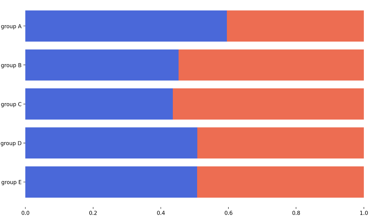
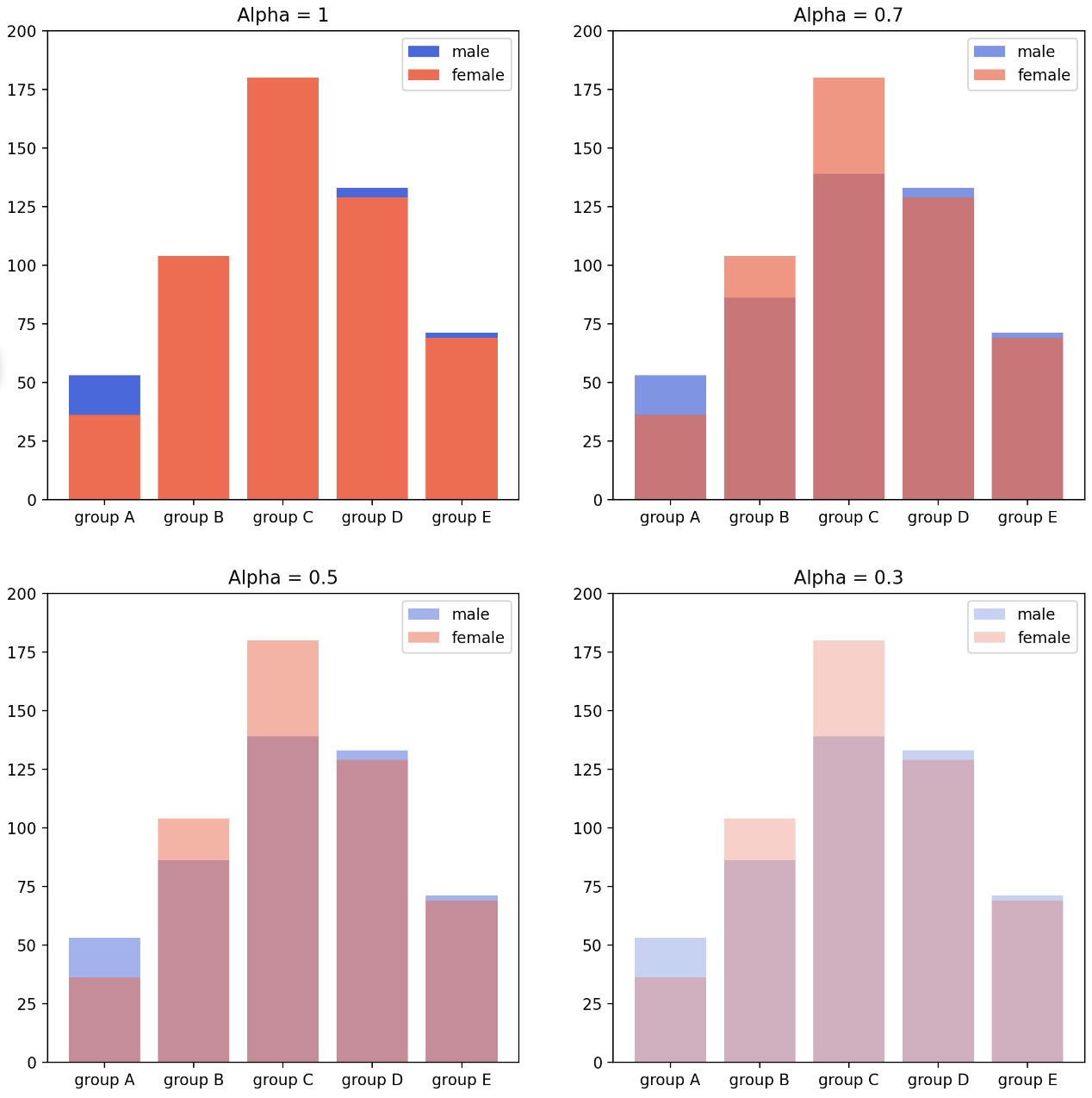
- Stacked bar plot 이 아닌 Overlapped bar plot 을 사용하면 변수 간 비교가 용이해진다.
.bar()내부에alpha로 투명도를 조정할 수 있다. 아래 예제를 보자.
group = group.sort_index()

fig, axes = plt.subplots(2, 2, figsize=(12, 12))
axes = axes.flatten() # 편한 indexing 을 위함

for idx, alpha in enumerate([1, 0.7, 0.5, 0.3]):
    axes[idx].bar(group['male'].index, group['male'], label='male',
                  color='royalblue',
                  alpha=alpha)
    axes[idx].bar(group['female'].index, group['female'], label='female',
                  color='tomato',
                  alpha=alpha)
    axes[idx].set_title(f'Alpha = {alpha}')

for ax in axes:
    ax.legend()
    ax.set_ylim(0, 200)

plt.show()
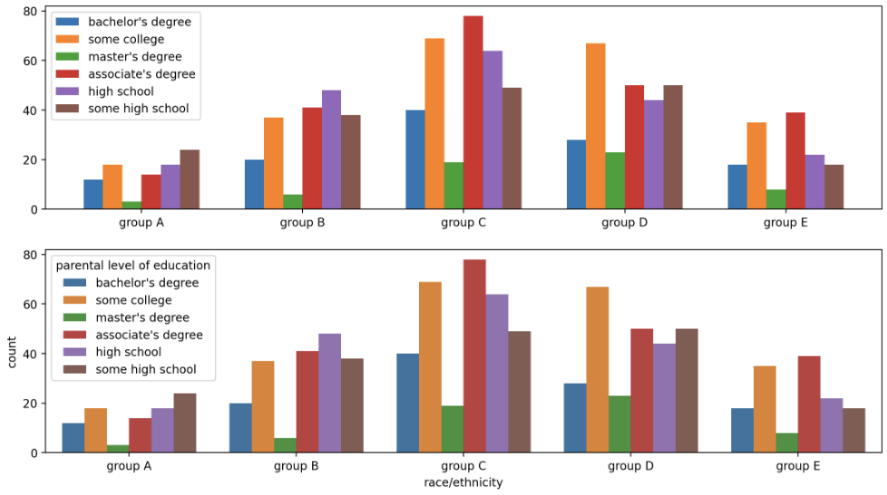
- 여러 변수를 비교할 때는 아래와 같이 x 축의 위치와
width를 이용하여 한눈에 비교할 수 있다. - 그러나 이 경우 x 축의 위치를 $x + \frac{-N+1+2\times i}{2} \times \text{witdh}$ 처럼 복잡하게 계산해야 하는데,
seaborn의 countplot 을 이용하면 쉽게 그릴 수 있다.
fig, axes = plt.subplots(2, 1, figsize=(13, 7))

x = np.arange(len(group_list))
width=0.12

for idx, g in enumerate(edu_lv):
    axes[0].bar(x+(-len(edu_lv)+1+2*idx)*width/2, group[g],
       width=width, label=g)

axes[0].set_xticks(x)
axes[0].set_xticklabels(group_list)
axes[0].legend()

axes[1] = sns.countplot(data=student, x='race/ethnicity', hue='parental level of education', order=sorted(student['race/ethnicity'].unique()))

plt.show()
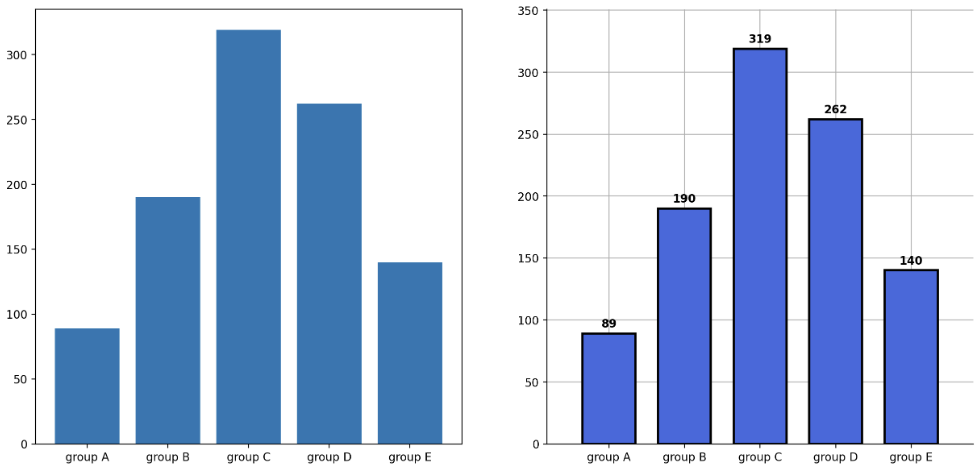
- 마지막으로 가독성을 올리기 위한 여러가지 테크닉을 사용할 수 있다. 각 주석을 참고하자.
group_cnt = student['race/ethnicity'].value_counts().sort_index()

fig = plt.figure(figsize=(15, 7))

ax_basic = fig.add_subplot(1, 2, 1)
ax = fig.add_subplot(1, 2, 2)

ax_basic.bar(group_cnt.index, group_cnt)
ax.bar(group_cnt.index, group_cnt,
       width=0.7,  # 두께 줄임
       edgecolor='black',   # 테두리 부각
       linewidth=2,  # 테두리 두께
       color='royalblue',
       zorder=10
      )

ax.margins(0.1, 0.1)  # 마진의 기본 디폴트값은 0.05, 즉 5%. 이를 10% 로

for s in ['top', 'right']:
    ax.spines[s].set_visible(False)  # 위, 오른쪽 변 제거해서 그래프를 개방적으로

ax.grid(zorder=0) # # 데이터가 어느 정도 스케일인지 잘 알 수 있게 도와줌. 가독성을 고려해보자

# 텍스트 넣기
for idx, value in zip(group_cnt.index, group_cnt):
    ax.text(idx, value+5, s=value,
                 ha='center', # 위치
                 fontweight='bold'  # 폰트
                )

plt.show()
lineplot
.plot()을 이용하여 line plot 을 그릴 수 있다.- line plot 은 $x_1, x_2, \cdots$ 와 $y_1, y_2, \cdots$ 데이터를 사용하여 그리며, 이전 점 $(x_1, y_1)$ 에서 $(x_2, y_2)$ 로 잇고, $(x_2, y_2)$ 에서 $(x_3, y_3)$ 로 잇는 순차적인 선으로 구성된 그래프다.
fig, ax = plt.subplots(1, 1, figsize=(5, 5))

np.random.seed(97)
x = np.arange(7)
y = np.random.rand(7)

ax.plot(x, y)

plt.show()
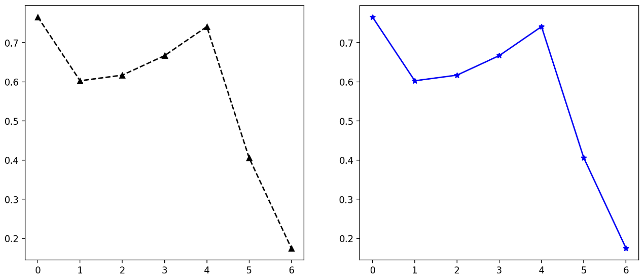
- 이 때
color,marker,linestyle을 가지고 line 을 다르게 그려줄 수 있다. 마커의 종류는 해당 링크에서 확인하자.
fig, axes = plt.subplots(1, 2, figsize=(12, 5))

x = np.arange(7)
y = np.random.rand(7)

axes[0].plot(x, y,
        color='black',
        marker='^',
        linestyle='--',
       )

axes[1].plot(x, y,
        color='blue',
        marker='*',
        linestyle='solid',
       )

plt.show()
- 뉴욕 주식 데이터를 가지고 line plot 을 좀 더 그려보자.
stock = pd.read_csv('./prices.csv')
stock['date'] = pd.to_datetime(stock['date'], format='mixed', errors='raise')
stock.set_index("date", inplace = True)

apple = stock[stock['symbol']=='AAPL']
google = stock[stock['symbol']=='GOOGL']
fig, ax = plt.subplots(1, 1, figsize=(15, 7), dpi=300)

ax.plot(google.index, google['close'])
ax.plot(apple.index, apple['close'])

plt.show()
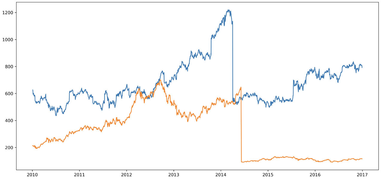
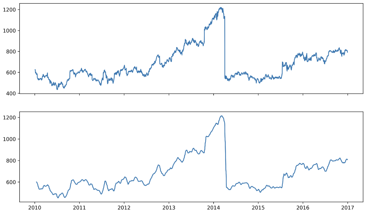
- 위 그래프를 보면 그래프에 노이즈가 많이 나타나므로
pandas의.rolling을 통해 이동평균을 계산하여 smoothing 해보자.
google_rolling = google.iloc[:,1:].rolling(window=10).mean()

fig, axes = plt.subplots(2, 1, figsize=(12, 7), dpi=300, sharex=True)

axes[0].plot(google.index,google['close'])
axes[1].plot(google_rolling.index,google_rolling['close']) # 이동평균 스무딩

plt.show()
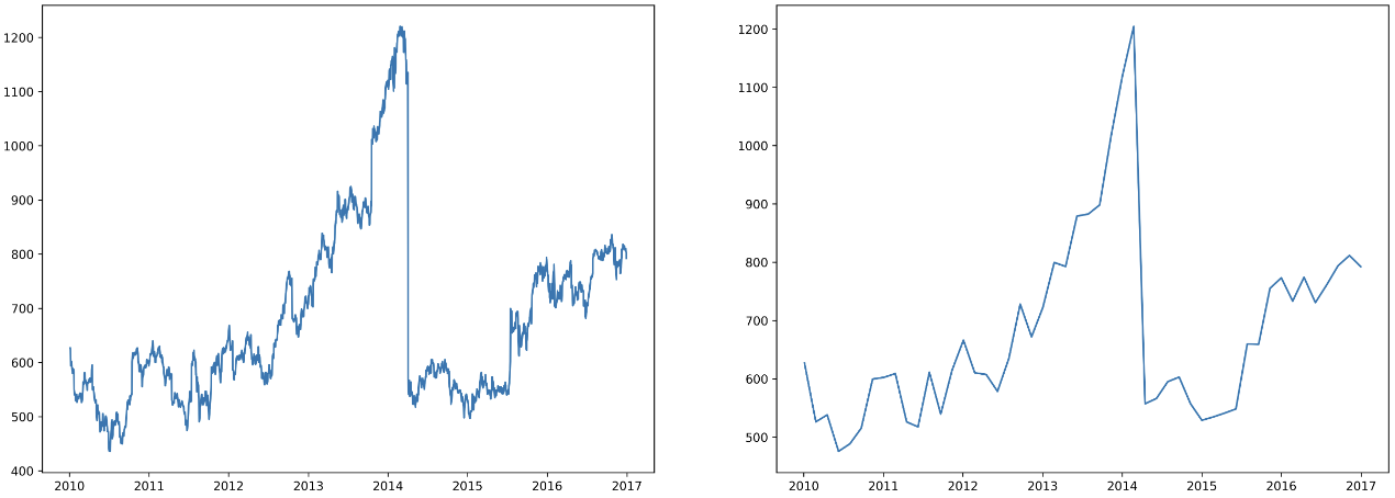
- 이렇게 그래프를 부드럽게 만드는 것은
scipy를 이용한 보간법으로도 가능하다.
from scipy.interpolate import make_interp_spline, interp1d
import matplotlib.dates as dates

fig, ax = plt.subplots(1, 2, figsize=(20, 7), dpi=300)

date_np = google.index
value_np = google['close']

date_num = dates.date2num(date_np)

# smooth
date_num_smooth = np.linspace(date_num.min(), date_num.max(), 50)
spl = make_interp_spline(date_num, value_np, k=3) # 스무딩
value_np_smooth = spl(date_num_smooth)

ax[0].plot(date_np, value_np)
ax[1].plot(dates.num2date(date_num_smooth), value_np_smooth)

plt.show()
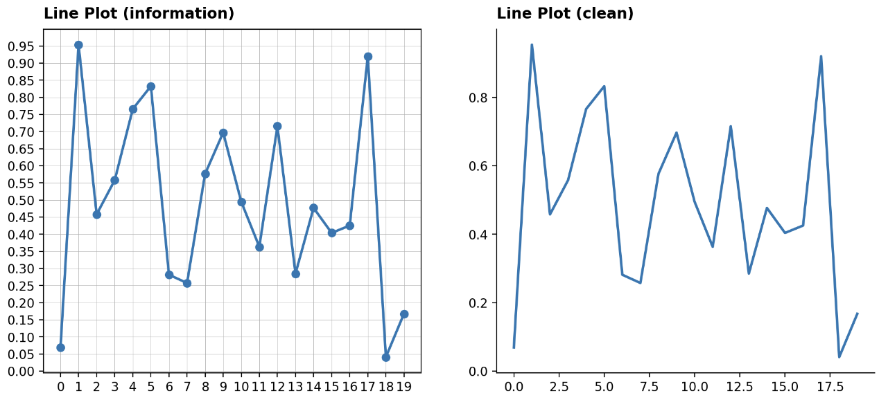
- 또한
matplotlob.ticker의MultipleLocator를 이용하면 좀 더 디테일하게 정보를 나타낼 수 있다. 아래에서 디테일하게 나타낸 정보와 간단하게 나타낸 정보를 비교해보자.
from matplotlib.ticker import MultipleLocator

fig = plt.figure(figsize=(12, 5))

np.random.seed(970725)

x = np.arange(20)
y = np.random.rand(20)

ax1 = fig.add_subplot(121)
ax1.plot(x, y,
         marker='o',
         linewidth=2)

ax1.xaxis.set_major_locator(MultipleLocator(1))  # 각 축에 대해 디테일하게
ax1.yaxis.set_major_locator(MultipleLocator(0.05))
ax1.grid(linewidth=0.3)

ax2 = fig.add_subplot(122)
ax2.plot(x, y,
       linewidth=2,)

ax2.spines['top'].set_visible(False)
ax2.spines['right'].set_visible(False)

ax1.set_title(f"Line Plot (information)", loc='left', fontsize=12, va='bottom', fontweight='semibold')
ax2.set_title(f"Line Plot (clean)", loc='left', fontsize=12, va='bottom', fontweight='semibold')

plt.show()
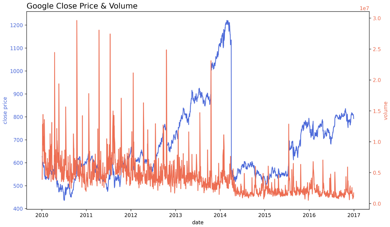
- 아래는
.twinx()를 통해 같은 Ax 에 다른 정보를 표현하는 예제다. 이 때 그래프의 색깔과 각 축의 색을 맞춰 한눈에 이해될 수 있도록 한다.
fig, ax1 = plt.subplots(figsize=(12, 7), dpi=150)

# First Plot
color = 'royalblue'

ax1.plot(google.index, google['close'], color=color)
ax1.set_xlabel('date')
ax1.set_ylabel('close price', color=color)
ax1.tick_params(axis='y', labelcolor=color)

# Second Plot
ax2 = ax1.twinx()  # 다른 정보를 표현
color = 'tomato'

ax2.plot(google.index, google['volume'], color=color)
ax2.set_ylabel('volume', color=color)
ax2.tick_params(axis='y', labelcolor=color)

ax1.set_title('Google Close Price & Volume', loc='left', fontsize=15)
plt.show()
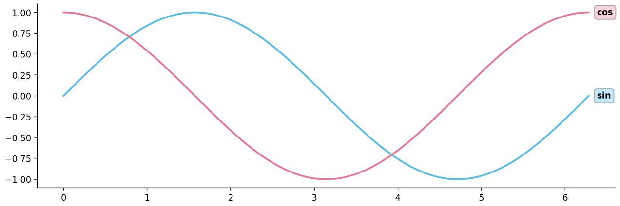
- 아래 예제는 line plot 에 어울리는 text 예제다.
fig = plt.figure(figsize=(12, 5))

x = np.linspace(0, 2*np.pi, 1000)
y1 = np.sin(x)
y2 = np.cos(x)

ax = fig.add_subplot(111, aspect=1) # aspact 는 subplot 의 가로/세로 scale 을 주어진 수의 비율로 맞춰주는 것
ax.plot(x, y1,
       color='#1ABDE9',
       linewidth=2,)

ax.plot(x, y2,
       color='#F36E8E',
       linewidth=2,)

# line plot 에 어울리는 각 line 우측 끝에 text 위치
ax.text(x[-1]+0.1, y1[-1], s='sin', fontweight='bold',
         va='center', ha='left',
         bbox=dict(boxstyle='round,pad=0.3', fc='#1ABDE9', ec='black', alpha=0.3))

ax.text(x[-1]+0.1, y2[-1], s='cos', fontweight='bold',
         va='center', ha='left',
         bbox=dict(boxstyle='round,pad=0.3', fc='#F36E8E', ec='black', alpha=0.3))

ax.spines['top'].set_visible(False)
ax.spines['right'].set_visible(False)

plt.show()
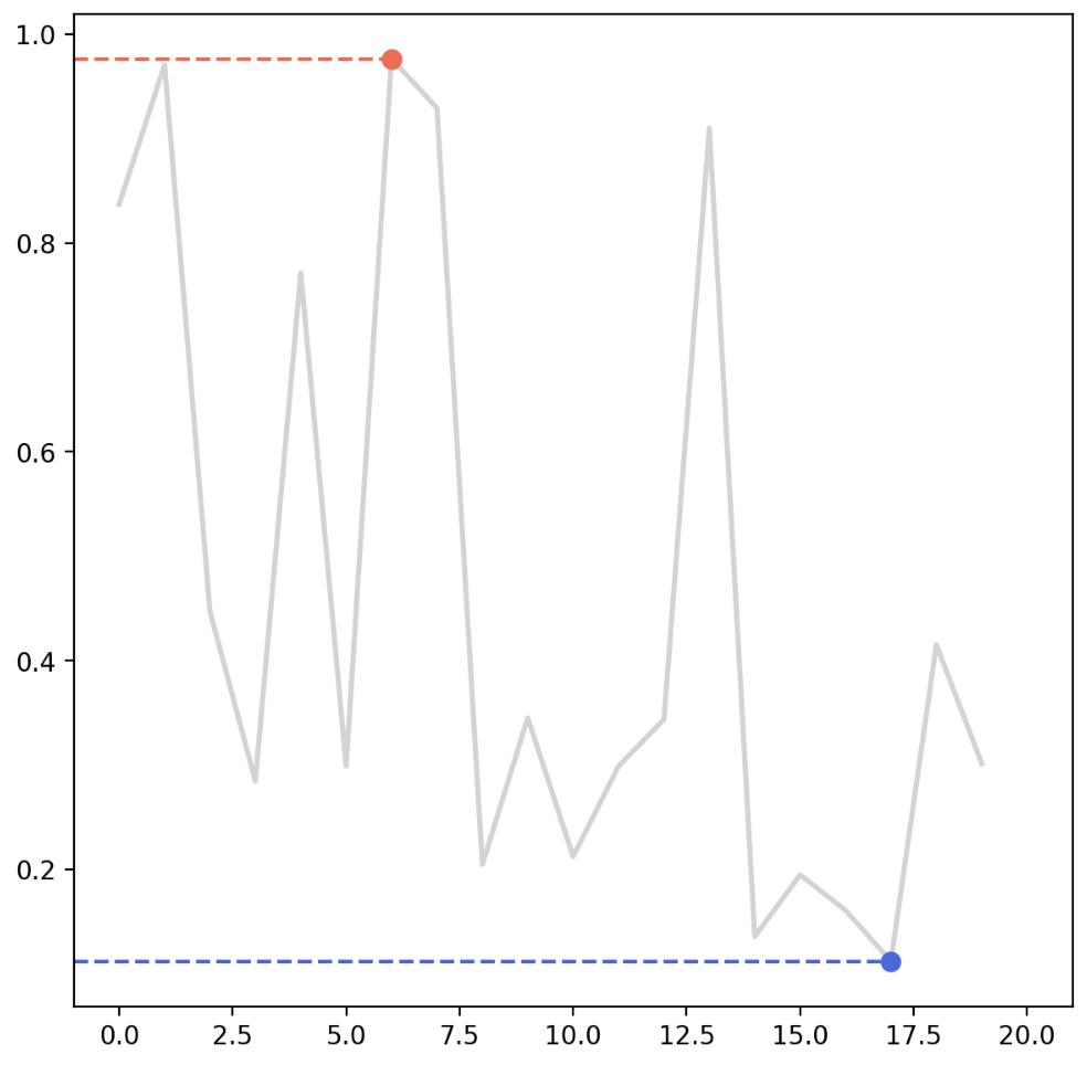
- 마지막으로 line plot 에서 해당 데이터의 최대값과 최소값을 같이 표시해주는 예제다.
fig = plt.figure(figsize=(7, 7))

np.random.seed(97)

x = np.arange(20)
y = np.random.rand(20)

ax = fig.add_subplot(111)
ax.plot(x, y,
       color='lightgray',
       linewidth=2,)

ax.set_xlim(-1, 21)

# max
ax.plot([-1, x[np.argmax(y)]], [np.max(y)]*2, linestyle='--', color='tomato')

ax.scatter(x[np.argmax(y)], np.max(y), c='tomato',s=50, zorder=20)

# min
ax.plot([-1, x[np.argmin(y)]], [np.min(y)]*2, linestyle='--', color='royalblue')
ax.scatter(x[np.argmin(y)], np.min(y), c='royalblue',s=50, zorder=20) # zorder 로 line graph 보다 위에 위치하도록 함.

plt.show()
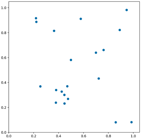
scatterplot
- scatter plot 은 점 $(x, y)$ 를 그래프 위에 나타낸다.
fig = plt.figure(figsize=(7, 7))
ax = fig.add_subplot(111, aspect=1)

x = np.random.rand(20)
y = np.random.rand(20)

ax.scatter(x, y)
ax.set_xlim(0, 1.05) # 위가 잘리는 부분이 있을 수 있으니 약간 높게
ax.set_ylim(0, 1.05)

plt.show()
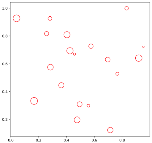
- scatter plot 도 마찬가지로 색(color), 모양(marker), 크기(size)를 지정하여 만들어줄 수 있다. 이 때 color 와 size 는 각각 배열로 전달하면 개별로 설정해줄 수 있다.
fig = plt.figure(figsize=(7, 7))
ax = fig.add_subplot(111, aspect=1)

np.random.seed(970725)

x = np.random.rand(20)
y = np.random.rand(20)
s = np.arange(20) * 20  # size

ax.scatter(x, y, s=s, c='white', marker='o', linewidth=1, edgecolor='red')
plt.show()
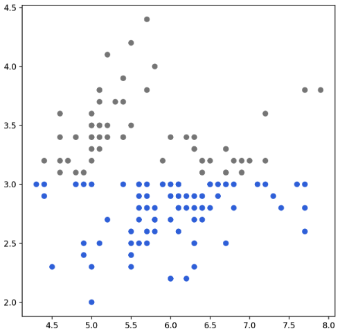
- iris 데이터를 가지고 scatter plot 을 그려보자. 이 때 색깔에 조건을 주어 원하는 정보를 얻을 수 있다.
fig = plt.figure(figsize=(7, 7))
ax = fig.add_subplot(111)

slc_mean = iris['SepalLengthCm'].mean()
swc_mean = iris['SepalWidthCm'].mean()

# 조건을 통해서 color 를 줄 수 있다.
ax.scatter(x=iris['SepalLengthCm'],
           y=iris['SepalWidthCm'],
           c=['royalblue' if yy <= swc_mean else 'gray' for yy in iris['SepalWidthCm']]
          )

plt.show()
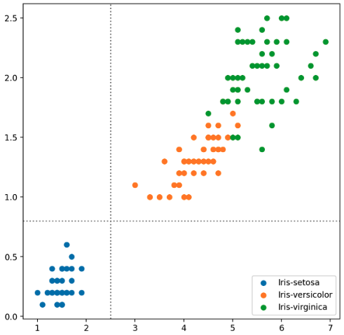
- 만약 변수들끼리 색으로 구분해야 한다면 같은 Ax 에 반복문으로 그려주는 것이 더 좋고 범례(
legend)를 사용하기에도 편리하다. 이를 통해 군집을 확인할 수 있다. - 또한 시각적인 주의를 주기 위하여 구분선을 그어줄 수도 있다.
fig = plt.figure(figsize=(7, 7))
ax = fig.add_subplot(111)

for species in iris['Species'].unique():
    iris_sub = iris[iris['Species']==species]
    ax.scatter(x=iris_sub['PetalLengthCm'],
               y=iris_sub['PetalWidthCm'],
               label=species)

# 구분선 사용하여 가독성 향상
ax.axvline(2.5, color='gray', linestyle=':')
ax.axhline(0.8, color='gray', linestyle=':')
ax.legend()
plt.show()
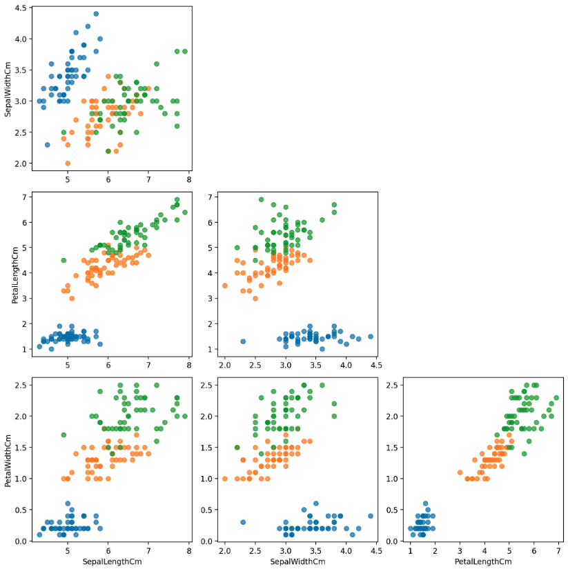
- 마지막으로 좀 더 다양한 관점에서 보기 위해 하나의 Figure 에 여러 Ax 를 두고, 거기에 변수를 다르게 하여 scatter plot 을 그릴 수 있다. 이는 Seabron 에서
pair plot을 사용하면 더 쉽게 가능하다. 그러나 변수가 많을 경우 시간이 오래 걸린다는 단점이 있다.
fig, axes = plt.subplots(4, 4, figsize=(14, 14))

feat = ['SepalLengthCm', 'SepalWidthCm', 'PetalLengthCm', 'PetalWidthCm']

for i, f1 in enumerate(feat):
    for j, f2 in enumerate(feat):
        if i <= j :
            axes[i][j].set_visible(False)  # sub plot 끄기
            continue
        for species in iris['Species'].unique():
            iris_sub = iris[iris['Species']==species]
            axes[i][j].scatter(x=iris_sub[f2],
                               y=iris_sub[f1],
                               label=species,
                               alpha=0.7)
        if i == 3: axes[i][j].set_xlabel(f2)
        if j == 0: axes[i][j].set_ylabel(f1)

plt.tight_layout()
plt.show()
text
- Matplotlib 에서 text 를 사용하여 좀 더 구체화된 정보를 나타낼 수 있다. 위에서
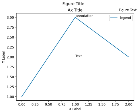
.text()와.annotate()를 잠깐 봤지만, 더 자세하게 보자. .suptitle,.set_title,.set_xlabel,.set_ylabel,.text,.annotate- Title 은 가장 큰 주제를 설명하고, Label 은 축에 해당하는 데이터 정보를 제공한다. Tick Label 은 축에 눈금을 사용하여 스케일 정보를 추가한다.
- Legend 는 한 그래프에서 2개 이상의 서로 다른 데이터를 분류하기 위해서 사용하는 보조 정보이며, Annotation(Text) 은 그 외의 시각화에 대한 설명을 추가하는데 사용한다.
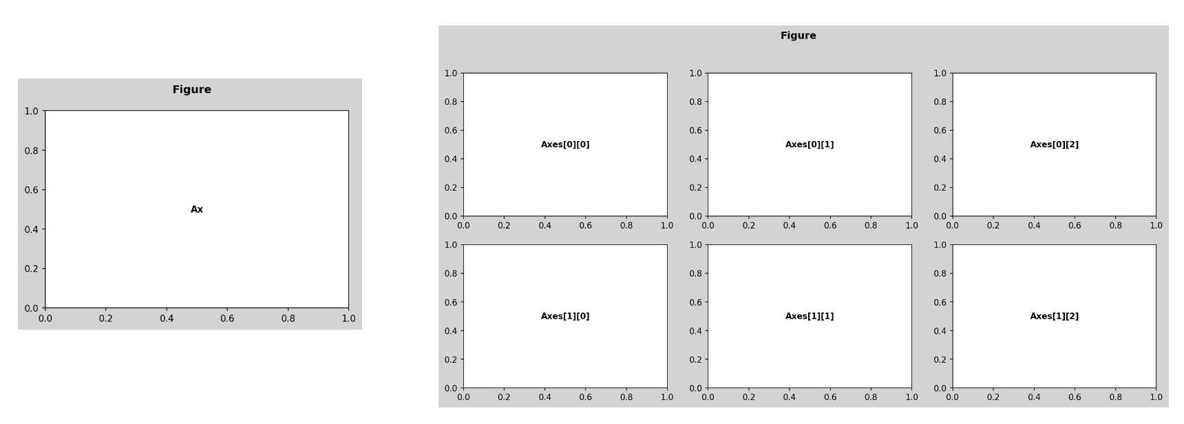
fig, ax = plt.subplots()

fig.suptitle('Figure Title')  # figure 의 타이틀

ax.plot([1, 3, 2], label='legend')
ax.legend()

ax.set_title('Ax Title') # ax 의 타이틀
ax.set_xlabel('X Label')
ax.set_ylabel('Y Label')

ax.text(x=1,y=2, s='Text') # ax 내 텍스트
fig.text(0.8, 0.9, s='Figure Text') # figure 내 텍스트. 비율로 위치
ax.annotate(text='annotation', xy=[1+.01, 3+.01])

plt.show()
-
.text에서 가독성을 위해 바꿔볼 수 있는 argument 로는fontfamily,fontsize,fontstyle,fontweight등이 있다.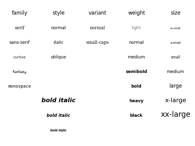
-
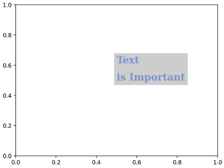
또한 폰트 자체말고도 커스텀할 수 있는 요소들이 있다.
color,linespacing,backgroundcolor,alpha,zorder,visible등이다.- 여기서
linespacing은 줄 간격을 뜻하고,alpha는 투명도,zorder는 z 축의 순서로 보이는 순서를 결정할 수 있다.
- 여기서
fig, ax = plt.subplots()
ax.set_xlim(0, 1)
ax.set_ylim(0, 1)

ax.text(x=0.5, y=0.5, s='Text\nis Important',
        fontsize='xx-large',
        fontweight='bold',
        fontfamily='serif',
        color='royalblue',
        linespacing=2,
        backgroundcolor='lightgray',
        alpha=0.5
       )

plt.show()
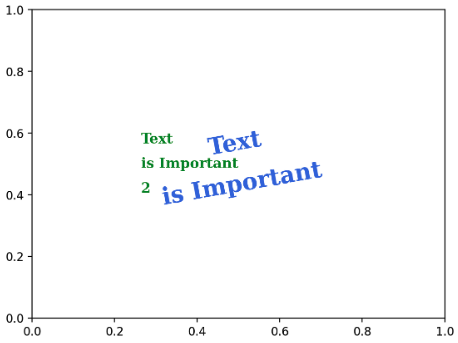
- 정렬과 관련하여 아래 요소들을 조정할 수 있다.
ha(horizontal alignment),va(vertical alignment),rotation,mulitalignment
fig, ax = plt.subplots()
ax.set_xlim(0, 1)
ax.set_ylim(0, 1)

ax.text(x=0.5, y=0.5, s='Text\nis Important',
        fontsize=20,
        fontweight='bold',
        fontfamily='serif',
        color='royalblue',
        linespacing=2,
        va='center', # top, bottom, center
        ha='center', # left, right, center
        rotation=10 # vertical. 숫자면 몇 도 회전할지,
       )

ax.text(x=0.5, y=0.5, s='Text\nis Important\n2',
        fontsize='large',
        fontweight='bold',
        fontfamily='serif',
        color='forestgreen',
        linespacing=2,
        va='center', # top, bottom, center
        ha='right', # left, right, center
        multialignment='left'
       )

plt.show()
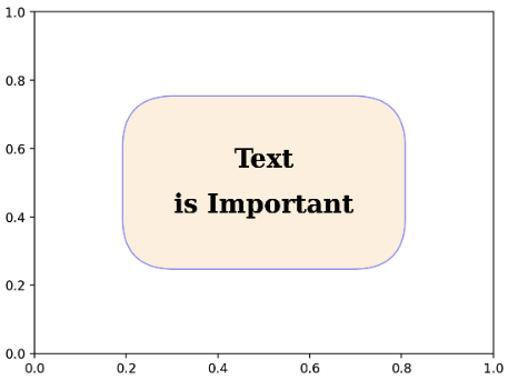
- text 에 box 를 씌워줄 수도 있다. box 의 종류는 matplotlib 의 공식문서를 확인하자.
fig, ax = plt.subplots()
ax.set_xlim(0, 1)
ax.set_ylim(0, 1)
ax.set_facecolor('white')
ax.text(x=0.5, y=0.5, s='Text\nis Important',
        fontsize=20,
        fontweight='bold',
        fontfamily='serif',
        color='black',
        linespacing=2,
        va='center', # top, bottom, center
        ha='center', # left, right, center
        rotation='horizontal', # vertical?
        bbox=dict(boxstyle='round', facecolor='wheat', alpha=0.4, edgecolor='blue', pad=2)  # dict 으로 찍어줘야 함.
       )

plt.show()
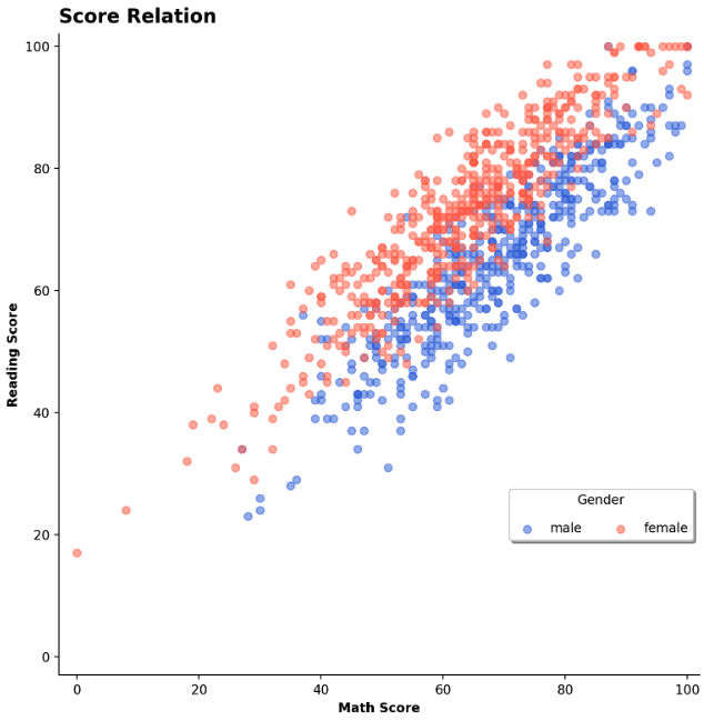
- 추가적으로 title 과 legend 의 경우
locarugment 도 위치를 지정해줄 수도 있다. 특히 legend 의 경우 legend 의 title, 그림자, 범례 라벨 간 간격, 컬럼 수 등 조정할 수 있다. - 아래 예제에서는 ax 의 title 을
loc을 통해 왼쪽으로 이동했고,legend에서bbox_to_anchor로 legend box 의 위치를 지정한 뒤loc을 통해 해당 지점이 box 의 어디에 위치하도록 할지 지정한 것이다.
fig = plt.figure(figsize=(9, 9))
ax = fig.add_subplot(111, aspect=1)

for g, c in zip(['male', 'female'], ['royalblue', 'tomato']):
    student_sub = student[student['gender']==g]
    ax.scatter(x=student_sub ['math score'], y=student_sub ['reading score'],
               c=c,
               alpha=0.5,
               label=g)

ax.set_xlim(-3, 102)
ax.set_ylim(-3, 102)

ax.spines['top'].set_visible(False)
ax.spines['right'].set_visible(False)

ax.set_xlabel('Math Score',
              fontweight='semibold')
ax.set_ylabel('Reading Score',
              fontweight='semibold')

# loc -> location
ax.set_title('Score Relation',
             loc='left', va='bottom',
             fontweight='bold', fontsize=15
            )
ax.legend(
    title='Gender',
    shadow=True,
    labelspacing=1.2,
    bbox_to_anchor=[1.0, 0.2],
    loc='lower right', # anchor 가 오른쪽 아래 꼭지점에 오도록
    ncol=2 # columns 수 조절
)

plt.show()
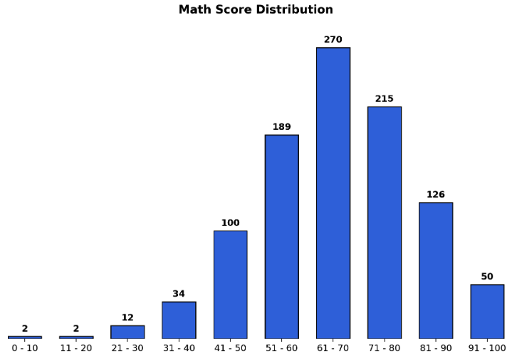
- 이제 bar plot 의 막대 위에 text 를 추가해보자. 추가적으로 아래 예제에서는 축을 제거하여 그래프가 더 눈에 잘 들어오도록 했다.
.set_xticks나.set_yticks에 빈 리스트를 주면 축이 제거된다. 그리고.set_xtickslabels를 통해 x 축의 표시 label 을 바꿔줄 수 있다..text에서y=val+3을 하여 실제 막대의 끝보다 좀 더 위에 text 를 위치시킨다.
# 막대 위에 텍스트 추가!
math_grade = student['math-range'].value_counts().sort_index()

fig, ax = plt.subplots(1, 1, figsize=(11, 7))
ax.bar(math_grade.index, math_grade,
       width=0.65,
       color='royalblue',
       linewidth=1,
       edgecolor='black'
      )

ax.margins(0.01, 0.1)
ax.set(frame_on=False) # ax 테두리 지우기
ax.set_yticks([])
ax.set_xticks(np.arange(len(math_grade)))
ax.set_xticklabels(math_grade.index, fontsize=11)

ax.set_title('Math Score Distribution', fontsize=14, fontweight='semibold')

for idx, val in math_grade.items():
    ax.text(x=idx, y=val+3, s=val,
            va='bottom',
            ha='center',
            fontsize=11, fontweight='semibold'
           )

plt.show()
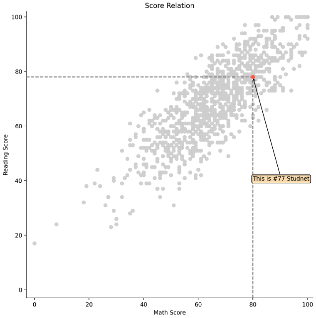
- 마지막으로
.annotate()에서 화살표를 이용해보자.
fig = plt.figure(figsize=(9, 9))
ax = fig.add_subplot(111, aspect=1)

i = 77

ax.scatter(x=student['math score'], y=student['reading score'],
           c='lightgray',
           alpha=0.9, zorder=5)

ax.scatter(x=student['math score'][i], y=student['reading score'][i],
           c='tomato',
           alpha=1, zorder=10)

ax.set_xlim(-3, 102)
ax.set_ylim(-3, 102)

ax.spines['top'].set_visible(False)
ax.spines['right'].set_visible(False)

ax.set_xlabel('Math Score')
ax.set_ylabel('Reading Score')

ax.set_title('Score Relation')

# x축과 평행한 선 -> x, y 가 각각 2개 원소가 있는 리스트인데, 이를 잘 맞춰보자!
ax.plot([-3, student['math score'][i]], [student['reading score'][i]]*2,
        color='gray', linestyle='--',
        zorder=8)

# y축과 평행한 선
ax.plot([student['math score'][i]]*2, [-3, student['reading score'][i]],
       color='gray', linestyle='--',
       zorder=8)

# 텍스트 bbox
bbox = dict(boxstyle="round", fc='wheat', pad=0.2)
# 화살표
arrowprops = dict(
    arrowstyle="->")

ax.annotate(text=f'This is #{i} Studnet',
            xy=(student['math score'][i], student['reading score'][i]), # 원하는 포인트의 위치
            xytext=[80, 40],  # 텍스트의 위치
            bbox=bbox,
            arrowprops=arrowprops,
            zorder=9
           )

plt.show()
color 와 facet
- 위치와 색은 가장 효과적인 채널 구분 수단이다. 위치는 시각화 방법에 따라 결정되고, 색은 우리가 직접적으로 골라야 한다.
- 이 때 주의해야 하는 것은 사람마다 색에 가지는 느낌은 다르다. 심미적으로 화려한 것은 분명 매력적이지만, 화려함은 시각화의 일부 요소일 뿐이다.
- 가장 중요한 것은 보는 사람에게 원하는 인사이트를 전달하는 것이고, 전하고 싶은 내용을 모두 전달했는가와 그 과정에서 오해는 없었는가가 중요하다.
- 색을 적재적소에 잘 사용하기 위해서 color palette 의 종류를 알면 좋다.
- 범주형(categorical) 데이터의 경우 독립된 색상으로 구성되어 색의 차이로 변수를 구분한다.
- 연속형(sequential) 데이터의 경우 정렬되고 연속적인 색상을 사용하여 값을 표현한다. 색상은 단일 색조로 표현하는 것이 좋다. github commit log (잔디)가 대표적 예시다.
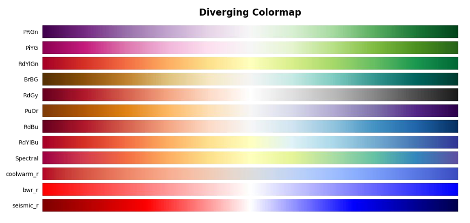
- 연속형과 유사하지만 중앙을 기준으로 발산하는 색을 사용할 수도 있다. 이 경우 기온과 같은 상반된 값이나 지지율과 같은 서로 다른 2개의 변수를 표현하는데 적합하다.
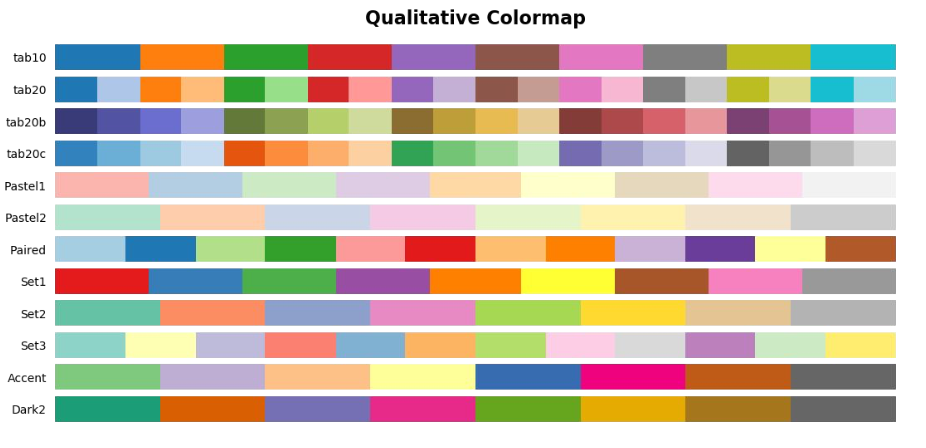

- 범주형 색상의 경우 일반적으로
tab10과Set2가 가장 많이 사용된다. matplotlib 에서는plt.cm.get_cmap으로 색을 받아올 수 있다. 아래 예제를 보자.
from matplotlib.colors import ListedColormap

qualitative_cm_list = ['Pastel1', 'Pastel2', 'Accent', 'Dark2', 'Set1', 'Set2', 'Set3', 'tab10']

fig, axes = plt.subplots(2, 4, figsize=(20, 8))
axes = axes.flatten()

student_sub = student.sample(100)

for idx, color in enumerate(qualitative_cm_list):
    pcm = axes[idx].scatter(student_sub['math score'], student_sub['reading score'],
                     c=student_sub['color'], cmap=ListedColormap(plt.cm.get_cmap(color).colors[:5])
                     )
    # 오른쪽에 있는 그룹 색깔 막대 그래프
    cbar = fig.colorbar(pcm, ax=axes[idx], ticks=range(5))
    cbar.ax.set_yticklabels(groups)
    axes[idx].set_title(color)

plt.show()
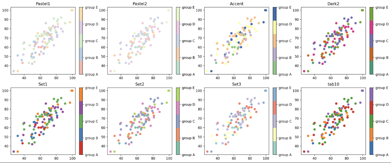
- 위 예제에서 사용된
fig.colorbar는 색마다 어떤 변수를 나타내는지 알려주는데 용이하다. - 연속형 색으로 github 잔디밭을 만들어보자.
im =  np.random.randint(10, size=(7, 52))
fig, ax = plt.subplots(figsize=(20, 10))
ax.imshow(im, cmap='Greens')
ax.set_yticks(np.arange(7)+0.5, minor=True)
ax.set_xticks(np.arange(52)+0.5, minor=True)
ax.grid(which='minor', color="w", linestyle='-', linewidth=3)
plt.show()
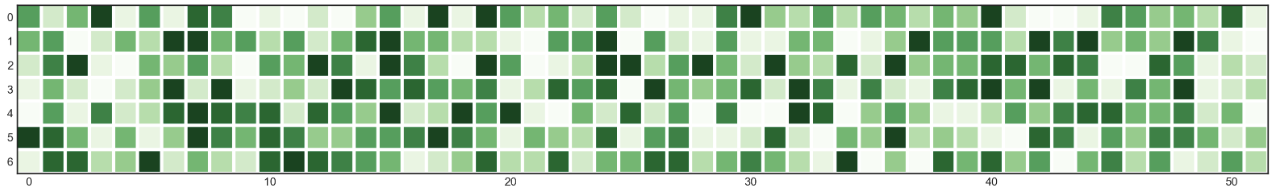
- 위 예제에서
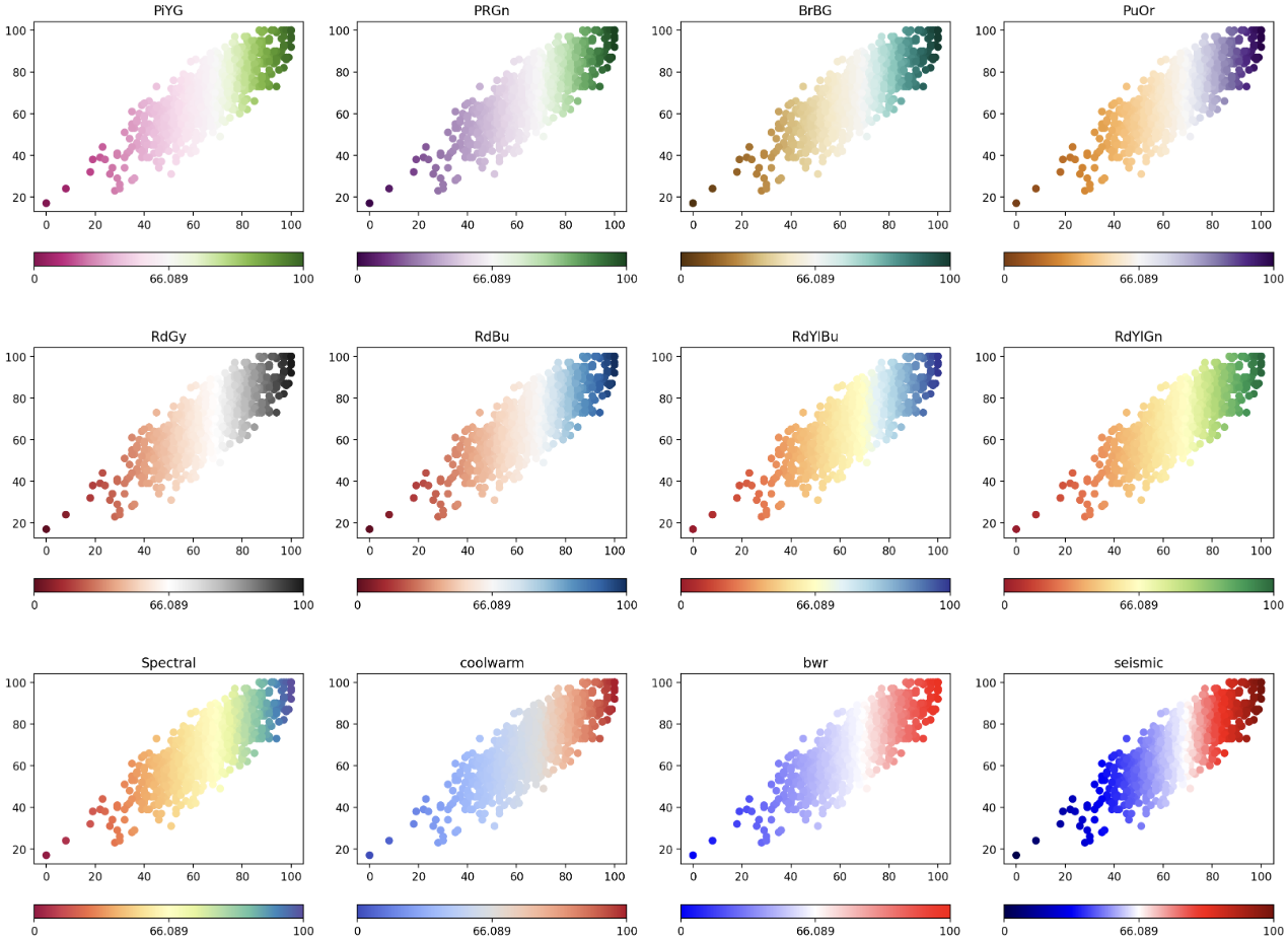
minor는 큰 격자와 세부 격자 중 세부 격자를 의미한다. - 발산형 색은 연속형과 거의 같지만, 어디를 중심으로 삼을 것인가가 중요하다. 평균에서 얼마나 떨어져있는가를 보기에 좋다.
matplotlib.colors에서TwoSlopeNorm은 발산형 색을 쓸 때 자주 사용하는 함수로, 중앙값을 정해주고 중앙값에 따른 비율로 바꿔준다.
from matplotlib.colors import TwoSlopeNorm

diverging_cm_list = ['PiYG', 'PRGn', 'BrBG', 'PuOr', 'RdGy', 'RdBu',
            'RdYlBu', 'RdYlGn', 'Spectral', 'coolwarm', 'bwr', 'seismic']

fig, axes = plt.subplots(3, 4, figsize=(20, 15))
axes = axes.flatten() # axes 는 넘파이 배열로 되어있다. 따라서 한 줄로 펴주면 반복문 사용에 용이하다.

offset = TwoSlopeNorm(vmin=0, vcenter=student['reading score'].mean(), vmax=100)
student_sub = student.sample(100)

for idx, cm in enumerate(diverging_cm_list):
    pcm = axes[idx].scatter(student['math score'], student['reading score'],
                            c=offset(student['math score']),
                            cmap=cm,
                     )
    cbar = fig.colorbar(pcm, ax=axes[idx],
                        ticks=[0, 0.5, 1],
                        orientation='horizontal'
                       )
    cbar.ax.set_xticklabels([0, student['math score'].mean(), 100])
    axes[idx].set_title(cm)

plt.show()
- 이 외에 특정 부분을 더 강조하기 위하여 색상 대비, 명도 대비, 채도 대비, 보색 대비 등을 사용할 수 있다. 이 경우
pandas의.apply메서드를 이용하여 기준에 따라 색을 다르게 하여 plot 을 만들 때 건네줄 수 있다.
a_color, nota_color = 'tomato', 'lightgreen'
colors = student['race/ethnicity'].apply(lambda x : a_color if x =='group A' else nota_color)
- Facet 이란 분할을 의미한다. 화면 상에 View 를 분할 및 추가하여 다양한 관점을 전달할 수 있다. 즉 같은 데이터셋에 서로 다른 인코딩을 통해 다른 인사이트를 전달할 수 있는 것이다.
- 같은 방법으로 동시에 여러 feature 를 보거나 큰 틀에서 볼 수 없는 부분 집합을 세세하게 보여줄 수 있다.
-
앞에서 봤듯 Figure 는 큰 틀, Ax 는 각 플롯이 들어가는 공간이다. 이 때 Figure 는 언제나 1 개이고, Ax(플롯)은 N 개가 된다.
- 서브 플롯을 만드는 가장 쉬운 방법은
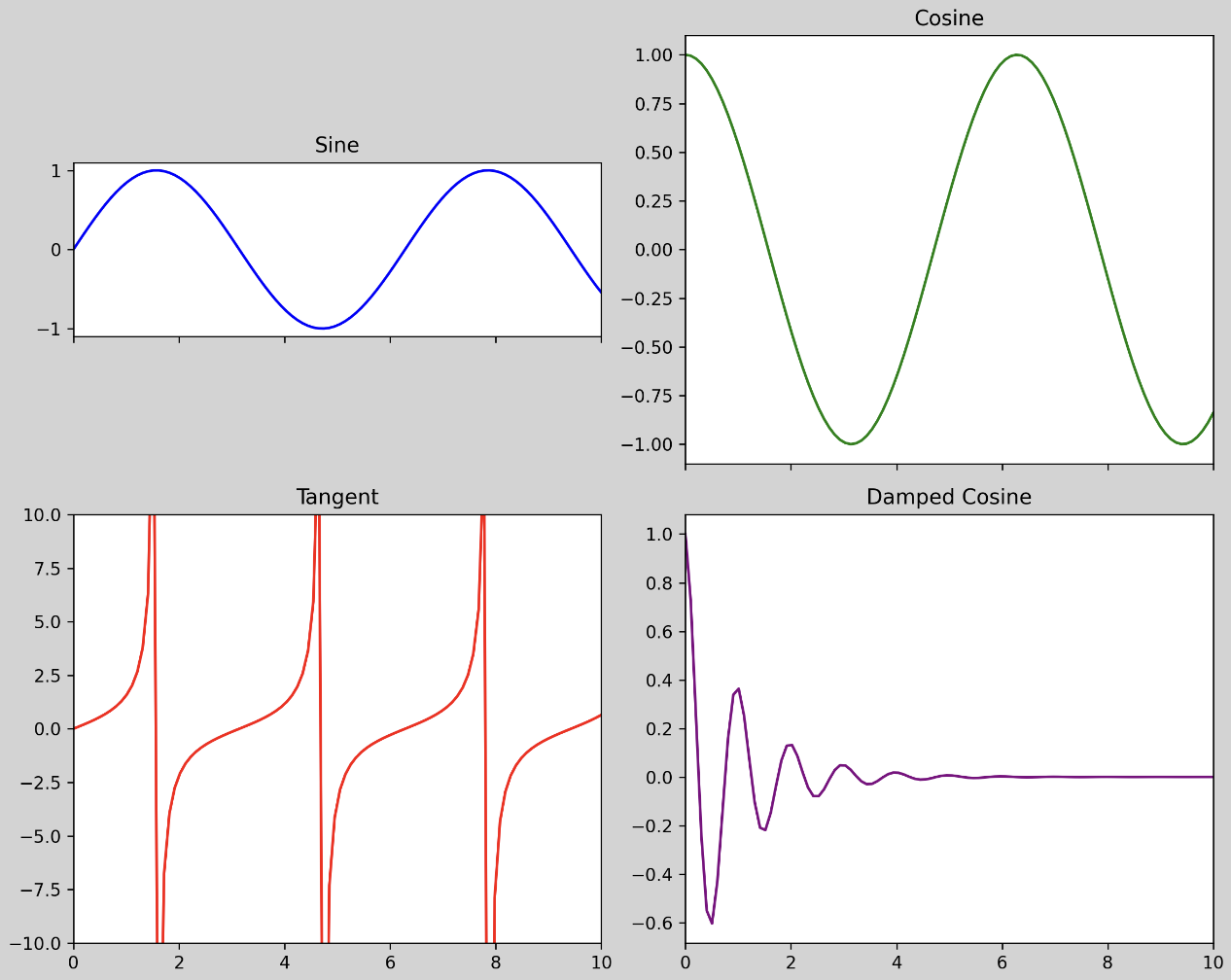
plt.subplot(),plt.figure() + fig.add_subplot(),plt.subplots()이다. 여기서 쉽게 조정할 수 있는 argument 는figsize, facecolor, dpi, sharex, sharey, squeeze, aspect등이 있다.fig.set_facecolor는 차트와 배경을 구분하기 위해 차트 배경 색을 조정하는 메서드다.dpi는 Dots per Inch 로 해상도를 의미하는 argument 다. 기본값은 100 이다.sharex, sharey는 서브 플롯을 사용할 때 개별 Ax 에 대해 축을 공유할 때 사용한다. 이를 통해 스케일 비교를 적합하게 할 수 있다.fig.add_subplot(122, sharey=ax1)이런 식으로 사용한다.squeeze는subplots()로 Ax 를 생성할 때 $n \times m$ 의 형태로numpy.ndarray타입의 Ax 배열이 생성된다. 이 때squeeze=False로 두면 2 차원으로 배열을 받을 수 있고 가변 크기에 대해 반복문을 사용하기 유용하다. 만약True라면 1 차원으로 flatten 된다.aspect는 x 축과 y 축의 비율을 의미한다. 즉aspect에 따라 Ax 의 크기가 다르게 나타나는데, 여기서set_xlim(), set_ylim()을 통해 다른 Ax 와 크기를 맞춰줄 수도 있다.
import matplotlib.pyplot as plt
import numpy as np

# 데이터 생성
x = np.linspace(0, 10, 100)
y1 = np.sin(x)
y2 = np.cos(x)
y3 = np.tan(x)
y4 = np.exp(-x) * np.cos(2 * np.pi * x)

# 서브 플롯 생성
fig, axs = plt.subplots(2, 2, figsize=(10, 8), dpi=120, sharex=True, sharey=False, squeeze=False)
fig.set_facecolor('lightgrey')

# 각 서브 플롯에 데이터 플롯
axs[0, 0].plot(x, y1, color='b')
axs[0, 0].set_title("Sine")
axs[0, 1].plot(x, y2, color='g')
axs[0, 1].set_title("Cosine")
axs[1, 0].plot(x, y3, color='r')
axs[1, 0].set_title("Tangent")
axs[1, 1].plot(x, y4, color='purple')
axs[1, 1].set_title("Damped Cosine")

# 각 서브 플롯의 aspect 비율 설정 및 x, y 축 제한
axs[0, 0].set_aspect(aspect=1.5)
axs[0, 0].set_xlim(0, 10)
axs[1, 0].set_ylim(-10, 10)

# 플롯 간격 조정
plt.tight_layout()
plt.show()
- 우리가 서브 플롯을 만들 때 grid 형태로 만들게 되는데 여기서 slicing 과 좌표형태(
x, y, dx, dy) 를 사용하면 더욱 유기적인 형태의 서브 플롯을 만들 수 있다. 이를 위해fig.add_gridspec(n, m)을 이용한다.
fig = plt.figure(figsize=(8, 5))

gs = fig.add_gridspec(3, 3) # make 3 by 3 grid (row, col)

ax = [None for _ in range(5)] # list to save many ax for setting parameter in each

ax[0] = fig.add_subplot(gs[0, :])
ax[0].set_title('gs[0, :]')

ax[1] = fig.add_subplot(gs[1, :-1])
ax[1].set_title('gs[1, :-1]')

ax[2] = fig.add_subplot(gs[1:, -1])
ax[2].set_title('gs[1:, -1]')

ax[3] = fig.add_subplot(gs[-1, 0])
ax[3].set_title('gs[-1, 0]')

ax[4] = fig.add_subplot(gs[-1, -2])
ax[4].set_title('gs[-1, -2]')

for ix in range(5):
    ax[ix].set_xticks([]) # to remove x ticks
    ax[ix].set_yticks([]) # to remove y ticks

plt.tight_layout()
plt.show()
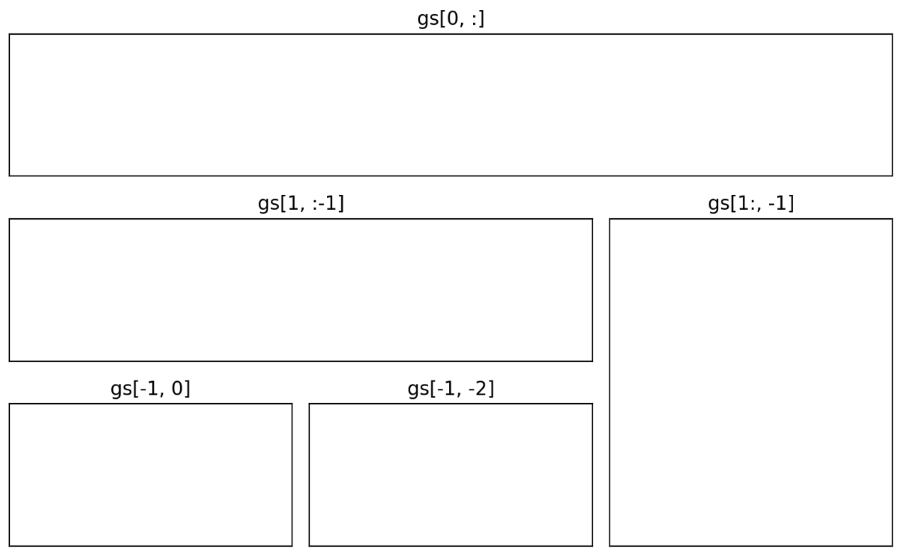
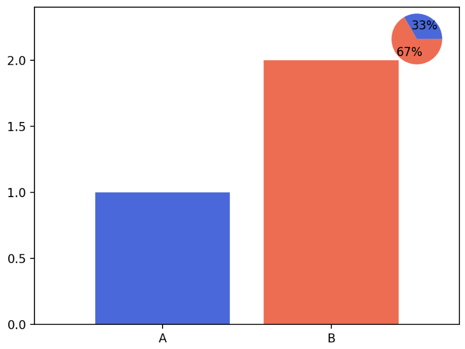
fig.add_axes([x, y, dx, dy])를 이용하면 특정 플롯을 임의의 위치에 만들수도 있다. 그러나 위치를 조정하여 그래프를 그리는 것이 쉽지는 않기 때문에 추천되지는 않는다.ax.inset_axes([x, y, dx, dy])는 미니맵 등 서브플롯 안에 원하는 서브플롯을 그릴 때 사용할 수 있다. 이는 표현하고자 하는 메인 시각화를 해치지 않는 선에서 사용하는 것이 좋다.
fig, ax = plt.subplots()

color=['royalblue', 'tomato']
ax.bar(['A', 'B'], [1, 2], color=color)

ax.margins(0.2)
axin = ax.inset_axes([0.8, 0.8, 0.2, 0.2])
axin.pie([1, 2], colors=color, autopct='%1.0f%%')
plt.show()
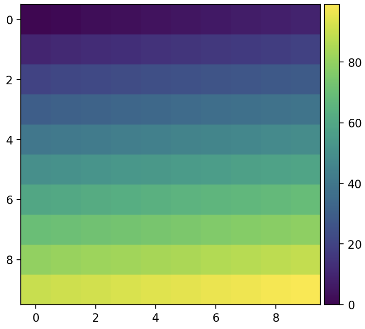
- 마지막으로 seaborn 에서는 argument 로
cbar를 줄 수 있는데, matplotlib 에서는 아래와 같이 colorbar 를 나타낼 수 있다.
from mpl_toolkits.axes_grid1.axes_divider import make_axes_locatable

fig, ax = plt.subplots(1, 1)

# 이미지를 보여주는 시각화. 2D 배열을 색으로 보여준다.
im = ax.imshow(np.arange(100).reshape((10, 10)))

divider = make_axes_locatable(ax)
cax = divider.append_axes("right", size="5%", pad=0.05)

fig.colorbar(im, cax=cax)
plt.show()
More Tips(grid, line, span, settings)
- matplotlib 에서 grid 는 아래와 같은 argument 를 가지고 있다.
which: major ticks, minor ticks, bothaxis: x 또는 y 축에 해당하는 grid 만 나타낼 수 있다. both 가 디폴트 값이다.color: grid 선의 색을 나타낸다.linestyle,linewidth: grid 선의 스타일과 두께zorder: plot 뒤에 위치하도록 사용한다. 0 이 되면 맨 뒤에 위치하게 된다.
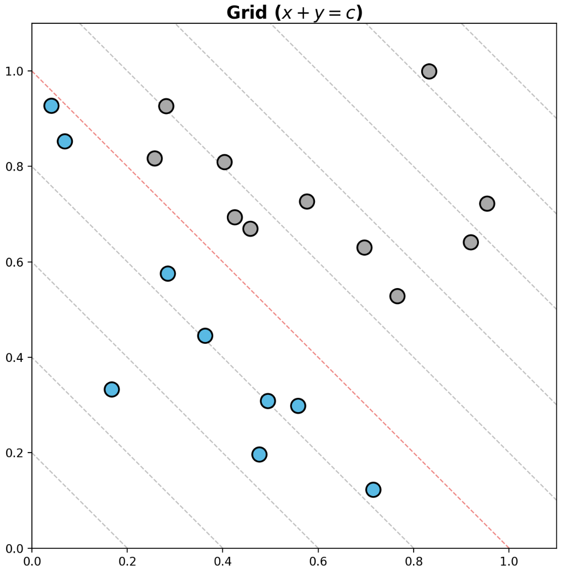
- 또한 grid 는
.grid말고도 일반적인 line plot.plot을 이용하여 grid 처럼 그려 사용할 수 있다. 아래는 대표적인 예제들이다.- 두 변수의 합이 중요하다면 $x + y = c$ 로 그릴 수 있다.
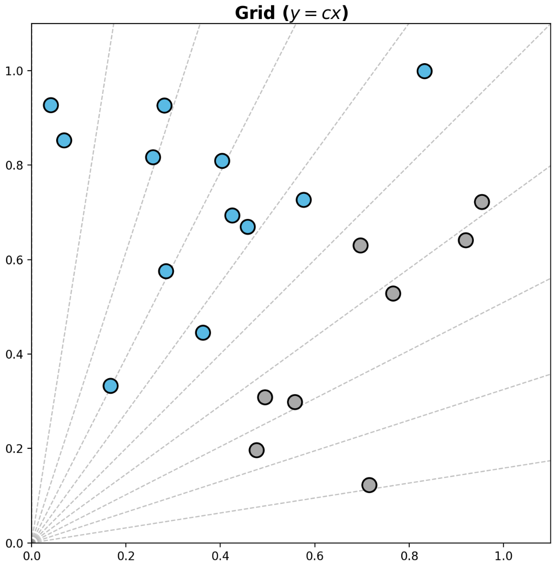
- 비율이 중요하다면 $y = cx$ 로 그릴 수 있다.
- 두 변수의 곱이 중요하다면 $xy = c$ 로 그릴 수 있다.
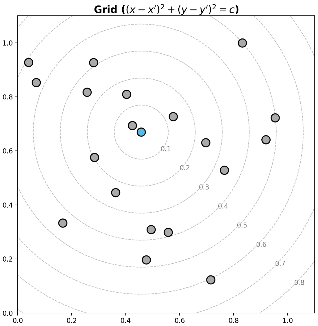
- 특정 데이터를 중심으로 보고 싶다면 $(x-x’)^2 + (y-y’)^2 = c$ 로 그릴 수 있다.
## x + y = c grid
x_start = np.linspace(0, 2.2, 12, endpoint=True)

for xs in x_start:
    ax.plot([xs, 0], [0, xs], linestyle='--', color='grey' if xs != 1.0 else 'red', alpha=0.5, linewidth=1)

## y = cx grid
radian = np.linspace(0, np.pi/2, 11, endpoint=True)

for rad in radian:
    ax.plot([0,2], [0, 2*np.tan(rad)], linestyle='--', color='gray', alpha=0.5, linewidth=1)

## 동심원 grid
rs = np.linspace(0.1, 0.8, 8, endpoint=True)

for r in rs:
    xx = r*np.cos(np.linspace(0, 2*np.pi, 100))
    yy = r*np.sin(np.linspace(0, 2*np.pi, 100))
    ax.plot(xx+x[2], yy+y[2], linestyle='--', color='gray', alpha=0.5, linewidth=1)

    ax.text(x[2]+r*np.cos(np.pi/4), y[2]-r*np.sin(np.pi/4), f'{r:.1}', color='gray')
- 이제 plot 에 선(line)과 면(span)을 추가할 수 있다.
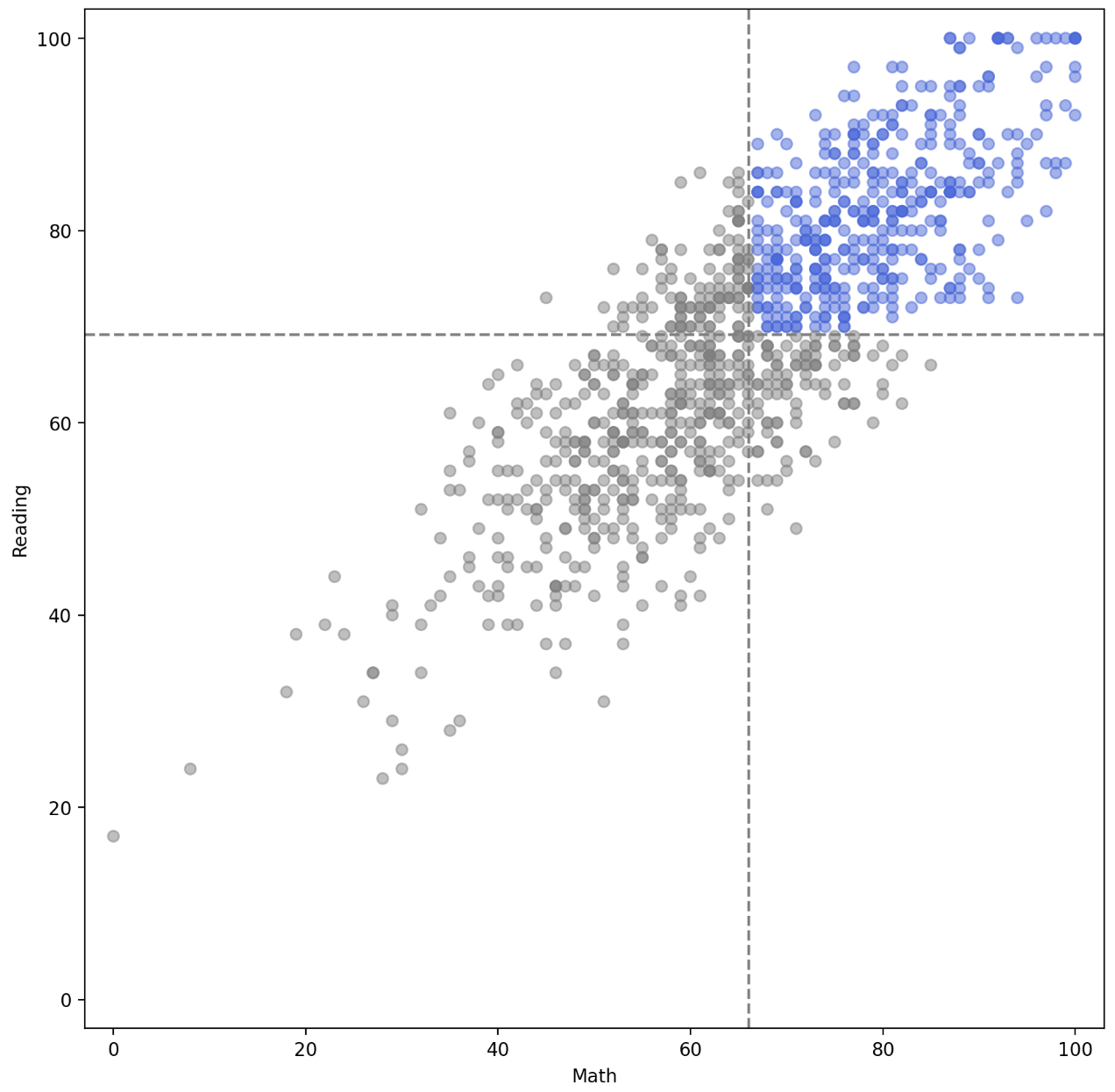
- 먼저
axvline(),axhline()을 통해 직교좌표계에서 평행선을 원하는 부분에 그릴 수 있다. 이를 통해 변수의 평균을 구하고 해당 값에 선을 그은 뒤, 해당 선 이상의 값을 색을 다르게 하여 plot 할 수 있다.
fig, ax = plt.subplots(figsize=(10, 10))
ax.set_aspect(1)

math_mean = student['math score'].mean()
reading_mean = student['reading score'].mean()

ax.axvline(math_mean, color='gray', linestyle='--')
ax.axhline(reading_mean, color='gray', linestyle='--')

ax.scatter(x=student['math score'], y=student['reading score'],
           alpha=0.5,
           color=['royalblue' if m>math_mean and r>reading_mean else 'gray'  for m, r in zip(student['math score'], student['reading score'])],
           zorder=10,
          )

ax.set_xlabel('Math')
ax.set_ylabel('Reading')

ax.set_xlim(-3, 103)
ax.set_ylim(-3, 103)
plt.show()
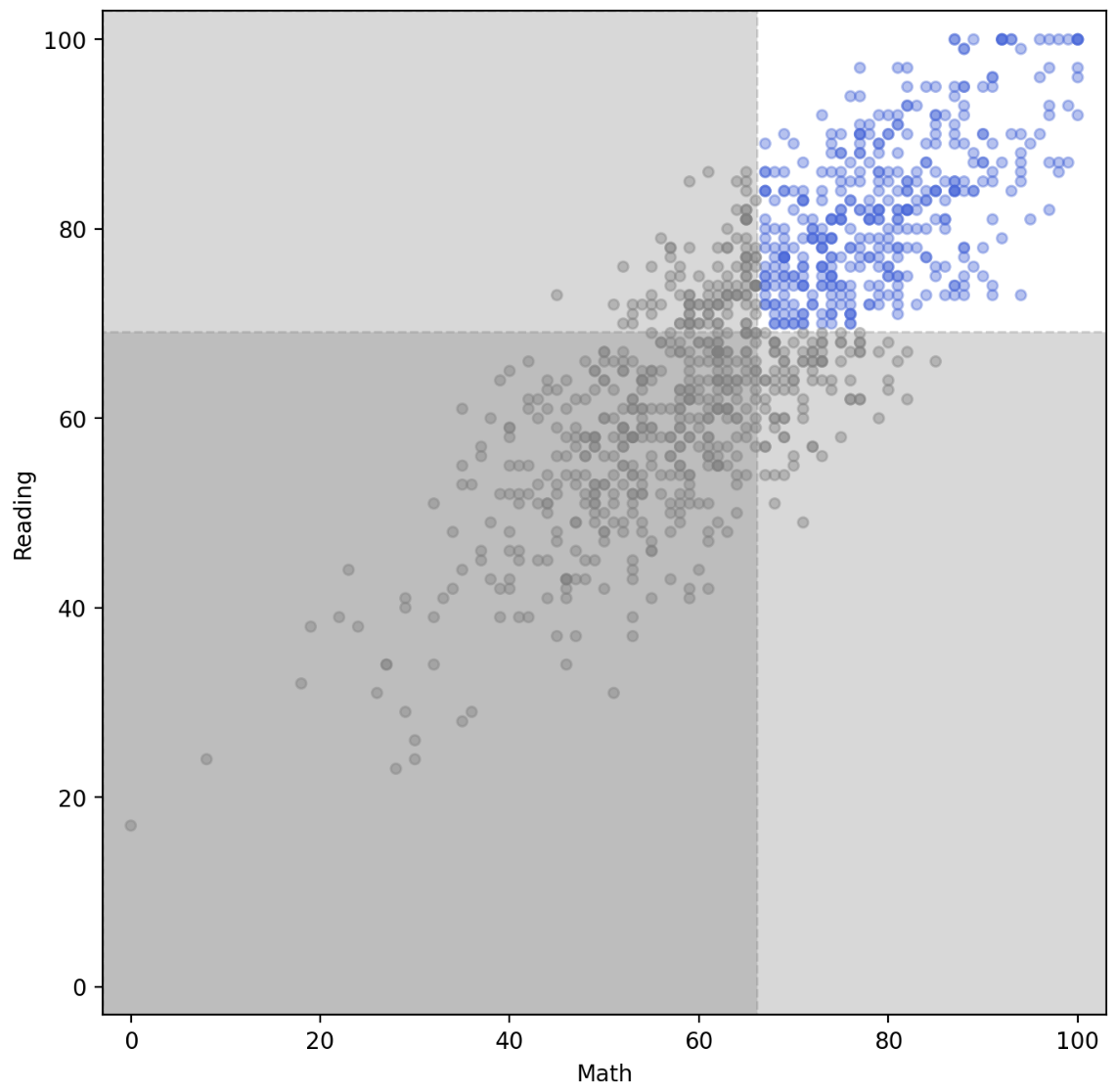
axvspan()과axhspan()을 이용하면 선과 함께 특정 부분의 면적을 표시할 수 있다. 이를 통해 특정 부분을 강조할 수도 있지만, 특정 부분의 주의를 없앨 수도 있다.
fig, ax = plt.subplots(figsize=(8, 8))
ax.set_aspect(1)

math_mean = student['math score'].mean()
reading_mean = student['reading score'].mean()

## 투명도 조정까지
ax.axvspan(-3, math_mean, color='gray', linestyle='--', zorder=0, alpha=0.3)
ax.axhspan(-3, reading_mean, color='gray', linestyle='--', zorder=0, alpha=0.3)

ax.scatter(x=student['math score'], y=student['reading score'],
           alpha=0.4, s=20,
           color=['royalblue' if m>math_mean and r>reading_mean else 'gray'  for m, r in zip(student['math score'], student['reading score'])],
           zorder=10,
          )

ax.set_xlabel('Math')
ax.set_ylabel('Reading')

ax.set_xlim(-3, 103)
ax.set_ylim(-3, 103)
plt.show()
- Spines 는 변을 뜻한다. 즉 Ax 의 4 변을 뜻한다. 여기에
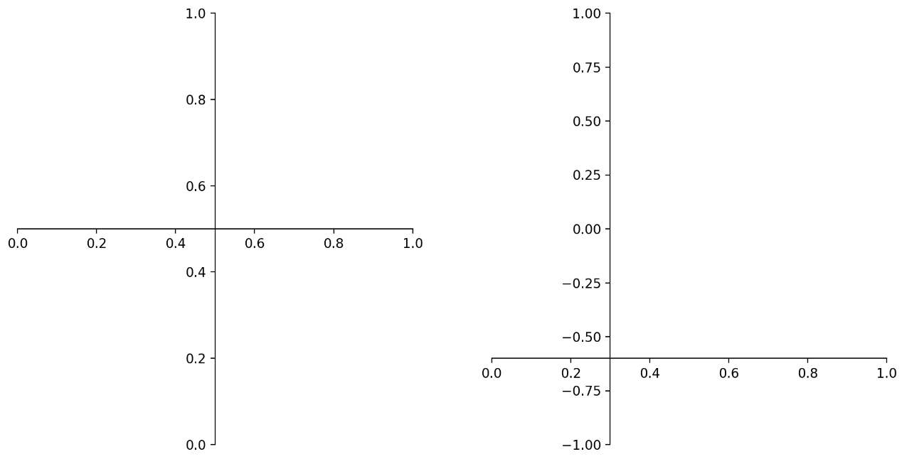
ax.spines.set_visible(),ax.spines.set_linewidth(),ax.spines.set_position()등을 이용할 수 있다. - 특히
ax.spines.set_position()를 이용하여 축을 중심 이외에 원하는 부분으로 옮길 수 있다.
fig = plt.figure(figsize=(12, 6))

ax1 = fig.add_subplot(1,2,1)
ax2 = fig.add_subplot(1,2,2)

for ax in [ax1, ax2]:
    ax.spines['top'].set_visible(False)
    ax.spines['right'].set_visible(False)

ax1.spines['left'].set_position('center')
ax1.spines['bottom'].set_position('center')

ax2.spines['left'].set_position(('data', 0.3)) # 0.3 에 해당하는 곳으로
ax2.spines['bottom'].set_position(('axes', 0.2))  # ax 의 비율

ax2.set_ylim(-1, 1)
plt.show()
- 마지막으로
plt.rcParams로 matplotlib pyplot 의 기본 설정을 바꿀 수 있고,print(mpl.style.available)에서 matplotlib 의 theme 을 바꿀 수도 있다. 해당 공식문서 페이지를 참고하자.
Seaborn
- Seaborn 은 Matplotlib 기반 통계 시각화 라이브러리로서, 통계 정보인 구성, 분포, 관계 등을 시각화할 수 있다. Matplotlib 기반이기 때문에 Matplotlib 으로 커스텀이 가능하며 쉬운 문법과 깔끔한 디자인이 특징이다.
- Seaborn 은 시각화의 목적과 방법에 따라 API 를 분류하여 제공하고 있다.
- Categorical API, Distribution API, Relational API, Regression API, Multiples API, Theme API
- 일반적으로 Seaborn 은
sns라는 별칭으로 import 한다.
import seaborn as sns
Count plot
countplot은 seaborn 의 Categorical API 에서 대표적인 시각화로 범주를 이산적으로 count 하여 막대 그래프로 그려주는 함수다.- 기본적으로 아래와 같은 argument 가 있다.
countplot(data=None, *, x=None, y=None, hue=None, order=None, hue_order=None, orient=None,
          color=None, palette=None, saturation=0.75, fill=True, hue_norm=None, stat='count',
          width=0.8, dodge='auto', gap=0, log_scale=None, native_scale=False, formatter=None, legend='auto', ax=None, **kwargs)
- 이 중
x,y,hue에는 기본적으로 pandas Dataframe 의 feature 를 넣어준다. - matplotlib 의 서브 플롯은
ax에 주면 된다. 그리고barh와 같이 방향을 바꾸는 방법은 전달되는 x 와 y 의 값을 바꾸면 된다. - 또한
order를 통해 데이터의 순서를 지정해줄 수 있다.
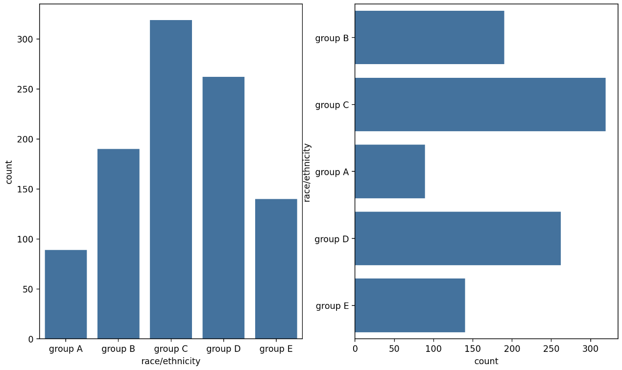
fig, axes = plt.subplots(1, 2, figsize=(12, 7))

sns.countplot(x='race/ethnicity', data=student, order=sorted(student['race/ethnicity'].unique()), ax=axes[0])
sns.countplot(y='race/ethnicity',data=student, ax=axes[1])

plt.show()
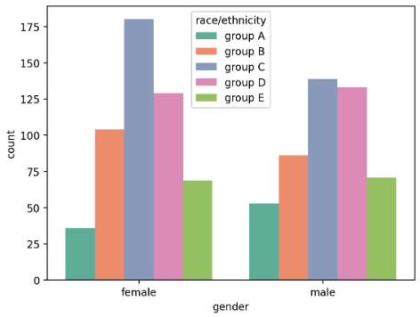
hue는 색을 의미하는데, 데이터의 구분 기준을 정하여 색상을 통해 내용을 구분한다. 이 때 색은palette를 변경하여 바꿀 수 있다. 만약color로 주게 된다면 연속형 색이 적용된다.- 이렇게 색으로 구분하게 될 때 순서가 애매해질 수 있는데, 이럴 때는
hue_order를 사용하여 순서를 정해준다.
sns.countplot(x='gender',data=student,
              hue='race/ethnicity',
              hue_order=sorted(student['race/ethnicity'].unique()), palette='Set2' #, color='red'
             )
Box plot
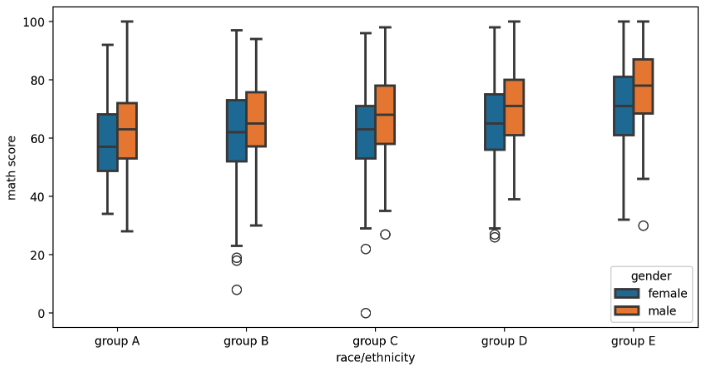
- 데이터의 분포를 살피는 대표적인 시각화 방법이다. 중간의 사각형은 25%(Q1), median(Q2), 75%(Q3) 값을 의미한다. 양 옆에 위치한 선은 whisker 라고 부르는데, 이 선을 넘어간 점들은 outlier 가 된다.
- 이 때의 whisker 들은 각각
Q1 - IQR * 1.5와Q3 + IQR * 1.5에 해당한다.
sns.boxplot(data=None, *, x=None, y=None, hue=None, order=None, hue_order=None, orient=None,
            color=None, palette=None, saturation=0.75, fill=True, dodge='auto', width=0.8, gap=0,
            whis=1.5, linecolor='auto', linewidth=None, fliersize=None, hue_norm=None,
            native_scale=False, log_scale=None, formatter=None, legend='auto', ax=None, **kwargs)
- 마찬가지로
hue를 주어 분포를 특정 key 에 따라 살펴볼 수 있다. 또한width,linewidth,fliersize로 시각화를 커스텀 할 수 있다.
fig, ax = plt.subplots(1,1, figsize=(10, 5))

sns.boxplot(x='race/ethnicity', y='math score', data=student,
            hue='gender',
            order=sorted(student['race/ethnicity'].unique()),
            width=0.3, # box 너비
            linewidth=2, # plot 선
            fliersize=8, # outlier 표시
            ax=ax)

plt.show()
Violin plot
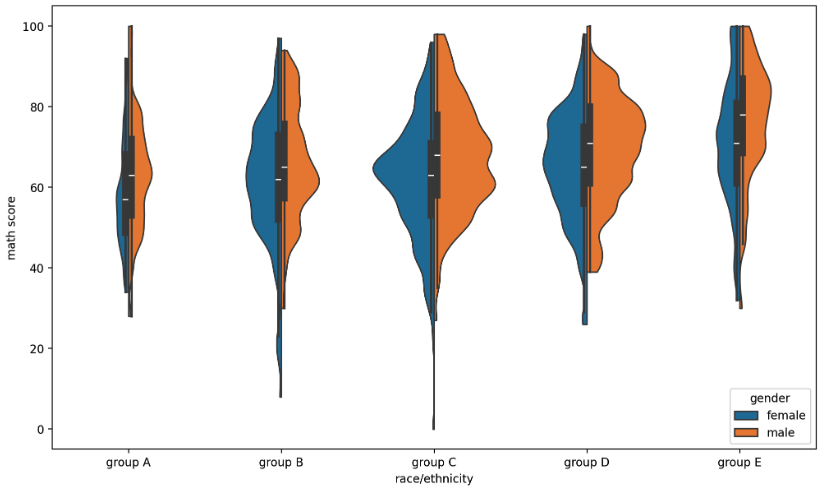
- box plot 은 대푯값을 잘 보여주지만 실제 분포를 표현하기에는 부족하다. 이 때 실제 분포에 대한 정보를 더 제공하기 위해 적합한 방식 중 하나가 Violin plot 이다.
- 가운데 선의 흰 점이 50% 를 나타내고, 중간 검정 막대가 IQR 범위를 의미한다. 그러나 이러한 violin plot 은 오해가 생길 수도 있다.
- violin plot 을 사용하는 데이터는 일반적으로 연속적이지 않고 kernel density estimate 를 사용하는데, 이와 같은 연속적 표현에서 생기는 데이터의 손실과 오차가 존재한다. 또한 데이터의 범위가 없는 데이터까지 표시된다.
- 이런 오해를 줄이고 정보량을 높이는 방법은 아래와 같다.
bw_method: 분포 표현을 얼마나 자세하게 보여줄 것인가,scott,silverman,floatcut: 끝부분을 얼마나 자를 것인가,floatinner_kws: 내부를 어떻게 표현할 것인가,box(box plot),quart(quartile),point(scatter),stick,None
sns.violinplot(data=None, *, x=None, y=None, hue=None, order=None, hue_order=None, orient=None,
              color=None, palette=None, saturation=0.75, fill=True, inner='box', split=False, width=0.8,
              dodge='auto', gap=0, linewidth=None, linecolor='auto', cut=2, gridsize=100,
              bw_method='scott', bw_adjust=1, density_norm='area', common_norm=False, hue_norm=None,
              formatter=None, log_scale=None, native_scale=False, legend='auto', scale=<deprecated>,
              scale_hue=<deprecated>, bw=<deprecated>, inner_kws=None, ax=None, **kwargs)
- 마찬가지로
hue를 사용하여 다양한 분포를 살펴볼 수 있고,density_norm을 통해 각 바이올린의 종류를 설정할 수 있다.split은 변수가 여러 개면 동시에 비교할 수 있게 해준다.
fig, ax = plt.subplots(1,1, figsize=(12, 7))
sns.violinplot(x='race/ethnicity', y='math score', data=student, ax=ax,
               order=sorted(student['race/ethnicity'].unique()),
               hue='gender',
               split=True,
               density_norm='count', # area, count, width
               bw_method=0.2, cut=0
              )
plt.show()
histplot
- 연속형 변수에 대해 히스토그램을 그린다. 이 때 막대 개수나 간격에 대한 조정은
binwidth와bins로 조정한다.
sns.histplot(data=None, *, x=None, y=None, hue=None, weights=None, stat='count', bins='auto',
            binwidth=None, binrange=None, discrete=None, cumulative=False, common_bins=True,
            common_norm=True, multiple='layer', element='bars', fill=True, shrink=1, kde=False,
            kde_kws=None, line_kws=None, thresh=0, pthresh=None, pmax=None, cbar=False, cbar_ax=None,
            cbar_kws=None, palette=None, hue_order=None, hue_norm=None, color=None, log_scale=None,
            legend=True, ax=None, **kwargs)
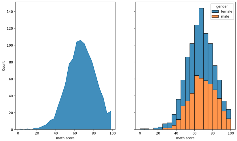
- 히스토그램은 기본적으로 막대지만, seaborn 에서는
elemnet를 통해 다른 표현들도 제공하고 있다. - 또한
stat을 통해 각 bin 을 나타내는 통계량을 나타낼 수 있고,multiple을 통해stack, layer, dodge, fill을 주어 N 개의 분포를 표현할 수 있다.
fig, axes = plt.subplots(1, 2, figsize=(12, 7), sharey=True)

sns.histplot(x='math score', data=student, ax=axes[0],
             stat='count', # 'count', 'density', 'percent', 'probability' or 'frequency'
             element='poly' # bars, step, poly
            )

sns.histplot(x='math score', data=student, ax=axes[1],
             binwidth=5,
             bins=100,
             hue='gender',
             multiple='stack', # layer, dodge, stack, fill
            )

plt.show()
kde plot
- Kernel Density Estimation(kde) 을 사용하여 분포를 나타낸다.
sns.kdeplot(data=None, *, x=None, y=None, hue=None, weights=None, palette=None, hue_order=None,
            hue_norm=None, color=None, fill=None, multiple='layer', common_norm=True, common_grid=False,
            cumulative=False, bw_method='scott', bw_adjust=1, warn_singular=True, log_scale=None,
            levels=10, thresh=0.05, gridsize=200, cut=3, clip=None, legend=True, cbar=False,
            cbar_ax=None, cbar_kws=None, ax=None, **kwargs)
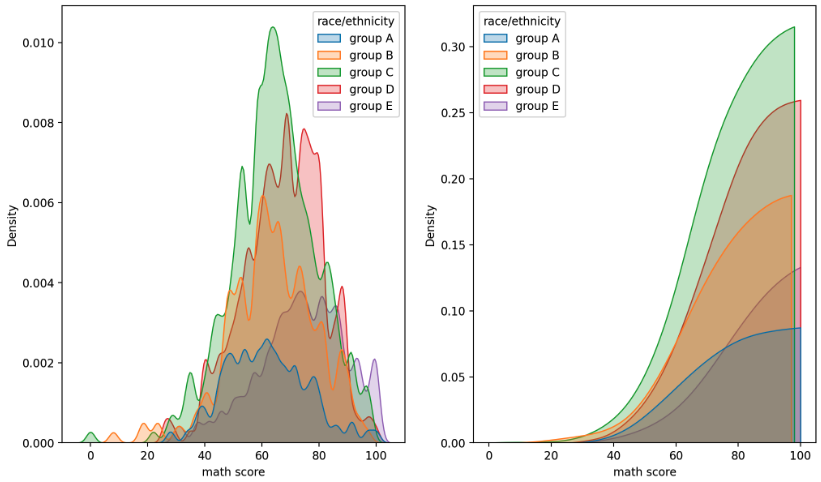
- 연속확률밀도를 보여주는 함수로 seaborn 의 다양한 smoothing 및 분포 시각화에 보조 정보로도 많이 사용한다. 실제로 위
histplot의 argument 중kde가 있다. - 밀도 함수를 그릴 때는 단순히 선만 그려서는 정보의 전달이 어려울 수 있다. 따라서
fill=True를 전달하여 내부를 채워 표현하는 것을 추천한다. bw_method를 사용하여 분포를 더 자세하게 표현할 수도 있다. 이러한 kde plot 은 histogram 의 연속적 표현이라고 생각하면 된다.cumulative는 누적분포를 나타낸다.
fig, axes = plt.subplots(1, 2, figsize=(12, 7))

sns.kdeplot(x='math score', data=student, ax=axes[0],
            fill=True,
            hue='race/ethnicity',
            hue_order=sorted(student['race/ethnicity'].unique()),
            bw_method=0.1)

sns.kdeplot(x='math score', data=student, ax=axes[1],
            fill=True,
            hue='race/ethnicity',
            hue_order=sorted(student['race/ethnicity'].unique()),
            multiple="layer", # layer, stack, fill
            cumulative=True,
            cut=0)

plt.show()
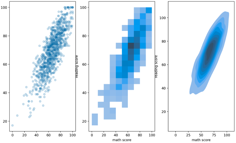
- hist plot 과 kde plot 에 2 개 변수를 사용할 수 있다. 이를 통해 결합 확률 분포(joint probability distribution)를 살펴볼 수 있다. 입력에 1 개의 축만 넣는 것이 아닌 2 개의 축 모두 입력으로 넣어주면 된다.
fig, axes = plt.subplots(1,3, figsize=(12, 7))

axes[0].scatter(student['math score'], student['reading score'], alpha=0.2)

sns.histplot(x='math score', y='reading score',
             data=student, ax=axes[1],
             cbar=False,
             bins=(10, 20),
            )

sns.kdeplot(x='math score', y='reading score',
            data=student, ax=axes[2],
            fill=True,
            )

plt.show()
ecdf plot, rug plot
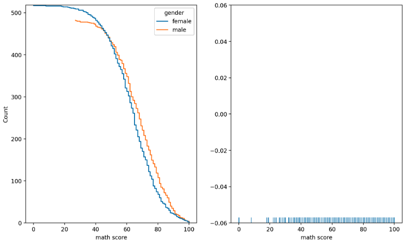
- ecdf plot 은 empirical cumulative distribution functions 을 나타낸다. 즉 누적되는 양을 표현한다. 이미 위에서
cumulative로 만들 수 있지만 따로 plot 이 존재한다. - rug plot 은 조밀한 정도를 통해 밀도를 나타낸다. 많이 사용되지는 않지만 한정된 공간 내에서 분포를 표현하기에는 좋다.
sns.ecdfplot(data=None, *, x=None, y=None, hue=None, weights=None, stat='proportion',
            complementary=False, palette=None, hue_order=None, hue_norm=None, log_scale=None,
            legend=True, ax=None, **kwargs)

sns.rugplot(data=None, *, x=None, y=None, hue=None, height=0.025, expand_margins=True, palette=None,
            hue_order=None, hue_norm=None, legend=True, ax=None, **kwargs)

fig, axes = plt.subplots(1, 2, figsize=(12, 7))
sns.ecdfplot(x='math score', data=student, ax=axes[0],
             hue='gender',
             stat='count', # proportion
             complementary=True # True 면 1-CDF(CCDF), False 면 CDF
            )
sns.rugplot(x='math score', data=student, ax=axes[1])
plt.show()
scatter plot
- matplotlib 에서 본 산점도 또한 seabron 에서 사용할 수 있다.
sns.scatterplot(data=None, *, x=None, y=None, hue=None, size=None, style=None, palette=None,
                hue_order=None, hue_norm=None, sizes=None, size_order=None, size_norm=None, markers=True,
                style_order=None, legend='auto', ax=None, **kwargs)
- 이 때
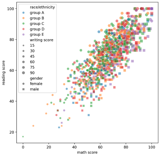
style,hue,size에 feature 들을 넣어 굉장히 많은 정보들을 표현할 수 있다. 아래 예제를 보자.
fig, ax = plt.subplots(figsize=(7, 7))
sns.scatterplot(x='math score', y='reading score', data=student,
                style='gender', markers={'male':'s', 'female':'o'},
                hue='race/ethnicity',
                hue_order=sorted(student['race/ethnicity'].unique()),
                size='writing score',
                alpha=0.5
               )
plt.show()
line plot
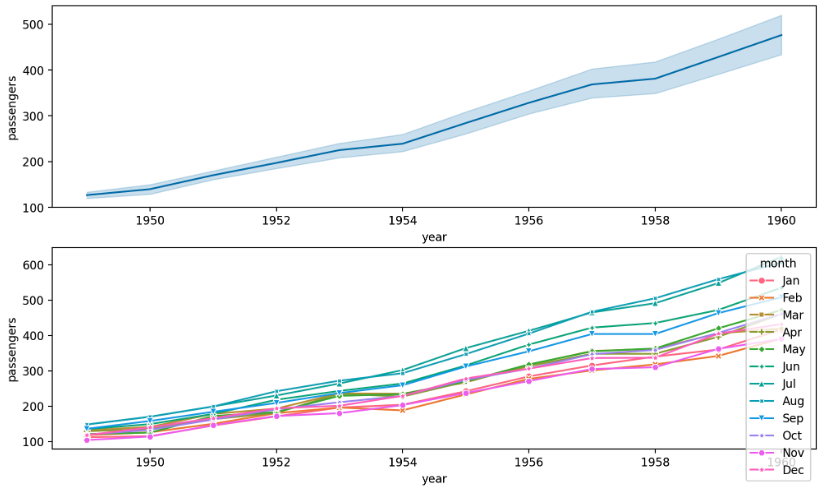
- seaborn 에서 line plot 은 자동으로 평균과 표준편차로 오차범위를 시각화 해준다. 또한 위와 마찬가지로
style,hue등을 이용하여 정보들을 표현할 수 있다.
sns.lineplot(data=None, *, x=None, y=None, hue=None, size=None, style=None, units=None, weights=None,
            palette=None, hue_order=None, hue_norm=None, sizes=None, size_order=None, size_norm=None,
            dashes=True, markers=None, style_order=None, estimator='mean', errorbar=('ci', 95),
            n_boot=1000, seed=None, orient='x', sort=True, err_style='band', err_kws=None, legend='auto',
            ci='deprecated', ax=None, **kwargs)

fig, axes = plt.subplots(2, 1, figsize=(12, 7))
sns.lineplot(data=flights, x="year", y="passengers", ax=axes[0])
sns.lineplot(data=flights, x="year", y="passengers", hue='month',
             style='month', markers=True, dashes=False,
             ax=axes[1])
plt.show()
reg plot
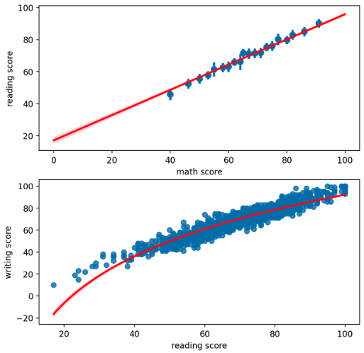
- 이는 회귀선을 추가한 scatter plot 이다.
sns.regplot(data=None, *, x=None, y=None, x_estimator=None, x_bins=None, x_ci='ci', scatter=True,
            fit_reg=True, ci=95, n_boot=1000, units=None, seed=None, order=1, logistic=False,
            lowess=False, robust=False, logx=False, x_partial=None, y_partial=None, truncate=True,
            dropna=True, x_jitter=None, y_jitter=None, label=None, color=None, marker='o',
            scatter_kws=None, line_kws=None, ax=None)
x_estimator을 사용하면 하나의 x 값의 한 개의 값만 보여줄 수 있으며np.mean을 사용하면 해당 x 에서의 분산도 확인할 수 있다. 또한x_bins를 통해 보여주는 개수도 지정할 수 있다.line_kws에dict형식으로 line 에 적용될 keywords 를 건네주면 회귀선의 색을 바꿀 수도 있다.order는 다차원 회귀선을 나타내고logx를 통해 로그를 사용할 수도 있다.
fig, axes = plt.subplots(2, 1, figsize=(7, 7))

sns.regplot(x='math score', y='reading score', data=student,
            x_estimator=np.mean, x_bins=20,
            line_kws=dict({"color":"red"}),
            ax=axes[0]
           )

sns.regplot(x='reading score', y='writing score', data=student,
            logx=True,
            ax=axes[1],
            line_kws=dict({"color":"red"}),
           )
plt.show()
heatmap
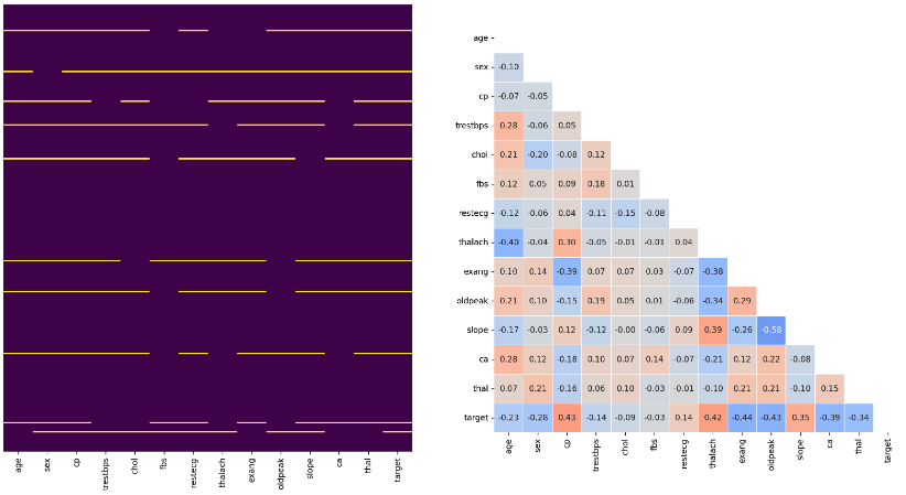
- 히트맵은 다양한 방식으로 사용될 수 있다. Dataframe 에서
nan값을 시각화하거나 상관관계 시각화에 많이 사용된다.
sns.heatmap(data, *, vmin=None, vmax=None, cmap=None, center=None, robust=False, annot=None, fmt='.2g',
            annot_kws=None, linewidths=0, linecolor='white', cbar=True, cbar_kws=None, cbar_ax=None,
            square=False, xticklabels='auto', yticklabels='auto', mask=None, ax=None, **kwargs)
- 상관계수는 -1 ~ 1 까지이므로 색의 범위를 맞추기 위해
vmin과vmax로 범위를 조정한다. 또한 0 을 기준으로 음/양이 중요하므로center를 지정해줄 수도 있다. cmap을 바꿔 가독성을 높일 수 있다. 상관관계는 음/양이 정반대의 의미를 가지기 때문에 diverse colormap 인coolwarm이 많이 사용된다.annot을 사용하면 heatmap 에 실제 상관관계 값이 들어가며,fmt를 통해 formatting 해줄 수 있다.- 또한
linewidth를 사용하면 칸 사이를 나눌 수 있고,square를 사용하면 정사각형이 되어 더 가독성이 좋아진다. - 추가로 상관관계 heatmap 의 경우 대칭인 경우가 많은데, 필요 없는 부분을 지우기 위해
np.triu를 mask 로 사용하기도 한다. cbar는 우측의 color bar 를 뜻하며False로 줄 경우 나오지 않는다.
fig, axes = plt.subplots(1,2 ,figsize=(20, 10))

sns.heatmap(heart_null.isnull(), yticklabels=False, cbar = False, cmap='viridis', ax=axes[0])

mask = np.triu(heart.corr())
sns.heatmap(heart.corr(), ax=axes[1], vmin=-1, vmax=1, center=0, cmap='coolwarm',
            annot=True, fmt='.2f',
            linewidth=0.1, square=True, cbar=False,
            mask=mask
           )
plt.show()
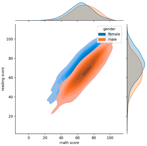
joint plot
- joint plot 은 2개 feature 의 결합 확률 분포와 함께 각각의 분포도 살필 수 있는 시각화를 제공한다.
sns.jointplot(data=None, *, x=None, y=None, hue=None, kind='scatter', height=6, ratio=5, space=0.2,
              dropna=False, xlim=None, ylim=None, color=None, palette=None, hue_order=None,
              hue_norm=None, marginal_ticks=False, joint_kws=None, marginal_kws=None, **kwargs)
- 이 때
kind에 따라 plot 안에 그려지는 것이 달라진다.
sns.jointplot(x='math score', y='reading score',data=student,
              hue='gender',
              kind='kde', # { “scatter” | “kde” | “hist” | “hex” | “reg” | “resid” },
              fill=True
             )
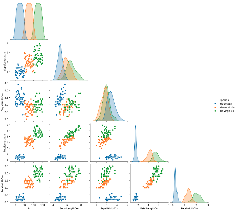
pair plot
- pair plot 은 데이터셋의 pair-wise 관계를 시각화하는 함수다.
sns.pairplot(data, *, hue=None, hue_order=None, palette=None, vars=None, x_vars=None, y_vars=None,
            kind='scatter', diag_kind='auto', markers=None, height=2.5, aspect=1, corner=False,
            dropna=False, plot_kws=None, diag_kws=None, grid_kws=None, size=None)
kind는 전체 서브플롯,diag_kind는 대각 서브플롯을 조정한다. 각각 {‘scatter’, ‘kde’, ‘hist’, ‘reg’}, {‘auto’, ‘hist’, ‘kde’, None} 가 가능하다.- 그리고 기본적으로 pair wise 하게 그리면 모양이 대각선을 기준으로 대칭인데,
corner를True로 하면 상삼각행렬의 plot 은 보지 않는다.
sns.pairplot(data=iris, hue='Species', kind='scatter', diag_kind='kde', corner=True)
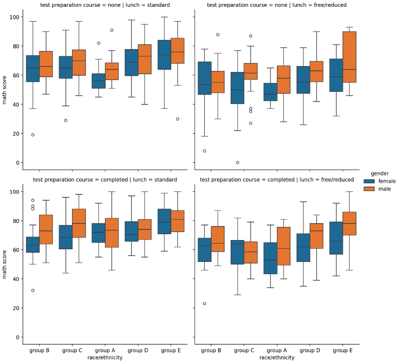
Facet Grid(catplot, displot, relplot, lmplot)
- 이 4 개의 plot 은 Facet Grid 를 기반으로 만들어졌으며 pairplot 과 같이 다중 패널을 사용하는 시각화를 의미한다.
- 다만 pair plot 은 feature-feature 사이를 살폈다면, Facet Grid 는 feature-feature 뿐 아니라 feature’s category-feature’s category 의 관계도 살펴볼 수 있다. 즉 row 와 column 에 따라 범주의 비교가 가능하다.
- 단일 시각화도 가능하지만, 여기서는 최대한 여러 pair 를 보며 관계를 살피는 것을 위주로 보자. 총 4개의 큰 함수가 Facet Grid 를 기반으로 만들어졌다.
catplot: Categoricaldisplot: Distributionrelplot: Relationallmplot: Regression
- catplot 은 아래의 방법론을 사용할 수 있다.
- Categorical scatterplots:
stripplot()(withkind="strip"; the default)swarmplot()(withkind="swarm")
- Categorical distribution plots:
boxplot()(withkind="box")violinplot()(withkind="violin")boxenplot()(withkind="boxen")
- Categorical estimate plots:
pointplot()(withkind="point")barplot()(withkind="bar")countplot()(withkind="count")
- Categorical scatterplots:
sns.catplot(data=None, *, x=None, y=None, hue=None, row=None, col=None, kind='strip', estimator='mean',
            errorbar=('ci', 95), n_boot=1000, seed=None, units=None, weights=None, order=None,
            hue_order=None, row_order=None, col_order=None, col_wrap=None, height=5, aspect=1,
            log_scale=None, native_scale=False, formatter=None, orient=None, color=None, palette=None,
            hue_norm=None, legend='auto', legend_out=True, sharex=True, sharey=True, margin_titles=False,
            facet_kws=None, ci=<deprecated>, **kwargs)
- 기본이 strip plot 이고, 다른 플롯도 사용할 수 있다. 또한 Facet Grid 는 행과 열을 조정하는 것이 중요하다.
row와col에는 categorical 변수를 넣어주면 된다.
sns.catplot(x="race/ethnicity", y="math score", hue="gender", data=student, kind='box',
            col='lunch', row='test preparation course')
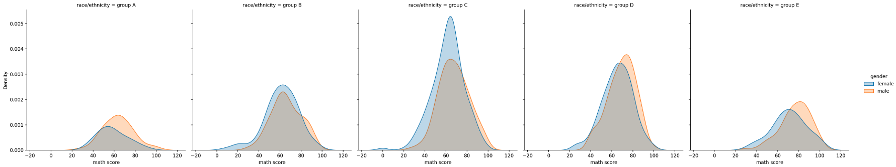
- displot 은 아래의 방법론을 사용할 수 있다.
histplot()(withkind="hist"; the default)kdeplot()(withkind="kde")ecdfplot()(withkind="ecdf"; univariate-only)
sns.distplot(a=None, bins=None, hist=True, kde=True, rug=False, fit=None, hist_kws=None, kde_kws=None,
             rug_kws=None, fit_kws=None, color=None, vertical=False, norm_hist=False, axlabel=None,
             label=None, ax=None, x=None)

sns.displot(x="math score", hue="gender", data=student,
           col='race/ethnicity', kind='kde', fill=True,
           col_order=sorted(student['race/ethnicity'].unique())
           )
- relplot 은 아래의 방법론을 사용할 수 있다.
scatterplot()(withkind="scatter"; the default)lineplot()(withkind="line")
sns.relplot(data=None, *, x=None, y=None, hue=None, size=None, style=None, units=None, weights=None,
row=None, col=None, col_wrap=None, row_order=None, col_order=None, palette=None,
hue_order=None, hue_norm=None, sizes=None, size_order=None, size_norm=None, markers=None,
dashes=None, style_order=None, legend='auto', kind='scatter', height=5, aspect=1,
facet_kws=None, **kwargs)
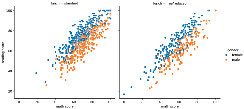
sns.relplot(x="math score", y='reading score', hue="gender", data=student, col='lunch')
- lmplot 은 아래의 방법론을 사용할 수 있다.
regplot()
sns.lmplot(data, *, x=None, y=None, hue=None, col=None, row=None, palette=None, col_wrap=None, height=5,
aspect=1, markers='o', sharex=None, sharey=None, hue_order=None, col_order=None,
row_order=None, legend=True, legend_out=None, x_estimator=None, x_bins=None, x_ci='ci',
scatter=True, fit_reg=True, ci=95, n_boot=1000, units=None, seed=None, order=1,
logistic=False, lowess=False, robust=False, logx=False, x_partial=None, y_partial=None,
truncate=True, x_jitter=None, y_jitter=None, scatter_kws=None, line_kws=None, facet_kws=None)
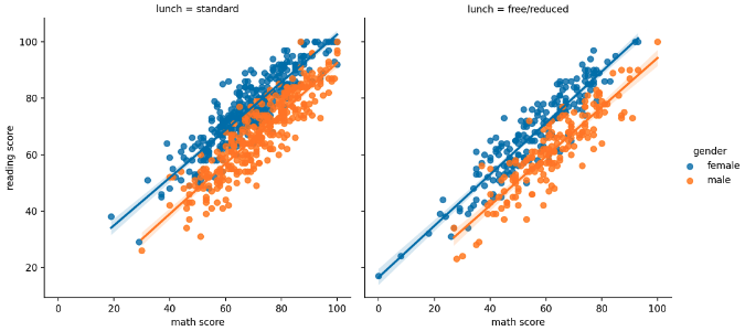
sns.lmplot(x="math score", y='reading score', hue="gender", data=student, col='lunch')
Polar Coordinate
- polar coordinate 는 극 좌표계이며, 서브플롯
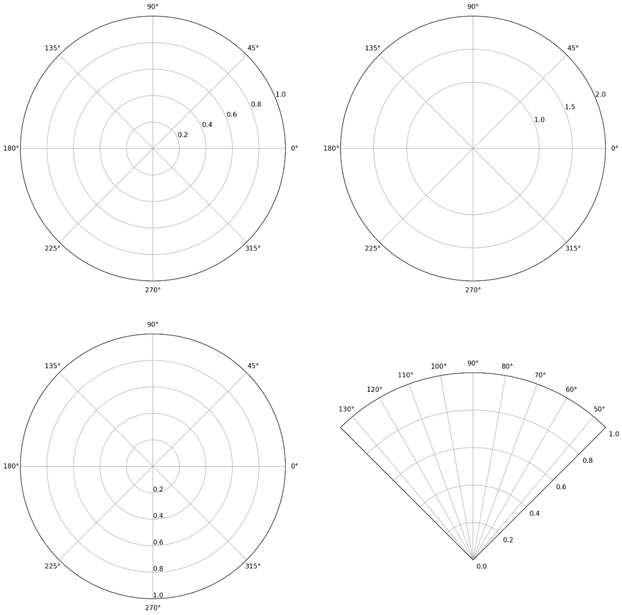
ax를 만들 때projection='polar'를 전달하거나polar=True를 주면 극 좌표계가 적용된 서브플롯을 그린다. set_rmax나set_rmin으로 반지름을 조정할 수 있고,set_rticks로 반지름 표기 grid 를 조정할 수 있다.set_rlabel_position은 반지름 label 이 적히는 위치의 각도를 조정한다.set_thetamin()과set_thetamax()는 각각 각도의 min 값과 max 값을 조정한다.
fig = plt.figure(figsize=(16, 16))

ax1 = fig.add_subplot(221, polar=True)

ax2 = fig.add_subplot(222, polar=True)
ax2.set_rmax(2)
ax2.set_rticks([1, 1.5, 2])

ax3 = fig.add_subplot(223, polar=True)
ax3.set_rlabel_position(-90)

ax4 = fig.add_subplot(224, polar=True)
ax4.set_thetamin(45)
ax4.set_thetamax(135)

plt.show()
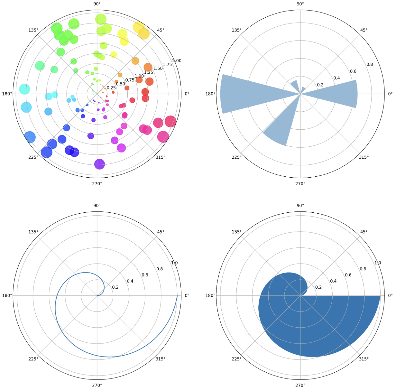
- scatter plot, bar plot, line plot 모두 사용할 수 있다.
np.random.seed(42)

fig = plt.figure(figsize=(16, 16))

## scatter
N = 100
r = 2 * np.random.rand(N)
theta = 2 * np.pi * np.random.rand(N)
area = 200 * r**2
colors = theta
ax = fig.add_subplot(221, projection='polar')
c = ax.scatter(theta, r, c=colors, s=area, cmap='hsv', alpha=0.75)

## bar
N = 6
r = np.random.rand(N)
theta = np.linspace(0, 2*np.pi, N, endpoint=False)
ax = fig.add_subplot(222, projection='polar')
ax.bar(theta, r, width=0.5, alpha=0.5)

## line
N = 1000
r = np.linspace(0, 1, N)
theta = np.linspace(0, 2*np.pi, N)
ax = fig.add_subplot(223, polar=True)
ax.plot(theta, r)

## fill
N = 1000
r = np.linspace(0, 1, N)
theta = np.linspace(0, 2*np.pi, N)
ax = fig.add_subplot(224, polar=True)
ax.fill(theta, r)

plt.show()
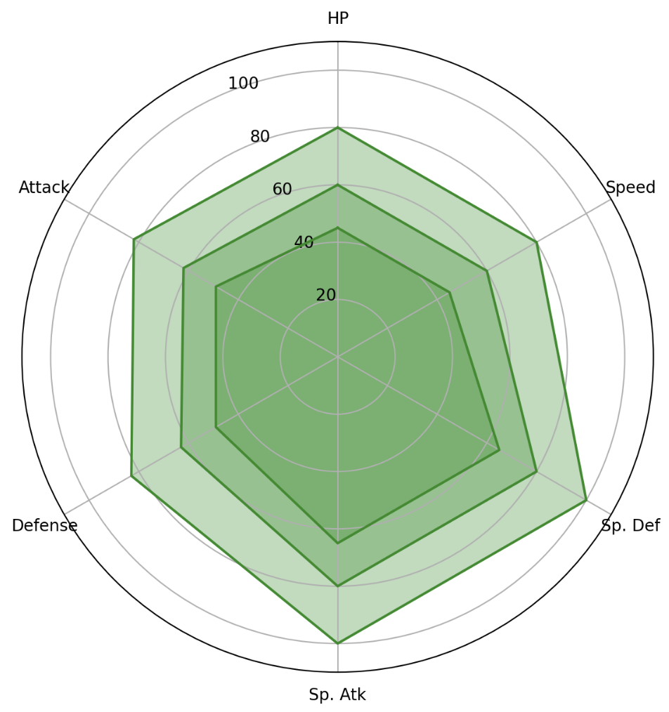
- 이러한 극 좌표계의
fill을 적절하게 이용하여 Rader Chart 를 그릴 수 있다. - 각은 $2\pi$ 를 6 등분 하고, value 와 함께 plot 을 그린 뒤
fill하면 된다. 여기서는 kaggle 의 포켓몬 데이터셋을 이용했다. set_thetagrids은 각도에 따른 그리드 및 ticklabels 를 변경하는데 사용된다.set_theta_offset은 시작 각도를 변경하는데 사용된다.
fig = plt.figure(figsize=(7, 7))
ax = fig.add_subplot(111, projection='polar')

theta = np.linspace(0, 2*np.pi, 6, endpoint=False)
theta = theta.tolist() + [theta[0]] # 끝 점 포함

for idx in range(3):
    values = pokemon.iloc[idx][stats].to_list()
    values.append(values[0])

    ax.plot(theta, values, color='forestgreen')
    ax.fill(theta, values, color='forestgreen', alpha=0.3)

ax.set_rmax(110)
ax.set_thetagrids([n*60 for n in range(6)], stats)
ax.set_theta_offset(np.pi/2)

plt.show()
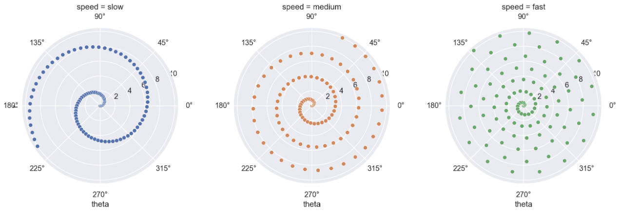
- seaborn 에서도
FacetGrid를 이용하여 극 좌표계를 이용할 수 있다. 서브 플롯을 그린 뒤.map으로 원하는 plot 을 적용시킨다.
# Generate an example radial datast
r = np.linspace(0, 10, num=100)
df = pd.DataFrame({'r': r, 'slow': r, 'medium': 2 * r, 'fast': 4 * r})

# Convert the dataframe to long-form or "tidy" format
df = pd.melt(df, id_vars=['r'], var_name='speed', value_name='theta')

# Set up a grid of axes with a polar projection
g = sns.FacetGrid(df, col="speed", hue="speed",
                  subplot_kws=dict(projection='polar'), height=4.5,
                  sharex=False, sharey=False, despine=False)

# Draw a scatterplot onto each axes in the grid
g.map(sns.scatterplot, "theta", "r")
pie
- seaborn 에는 없지만 matplotlib 에서는 pie chart 를 그릴 수 있다.
matplotlib.pyplot.pie(x, explode=None, labels=None, colors=None, autopct=None, pctdistance=0.6, shadow=False, labeldistance=1.1,
                      startangle=0, radius=1, counterclock=True, wedgeprops=None, textprops=None, center=(0, 0), frame=False,
                      rotatelabels=False, *, normalize=True, hatch=None, data=None)
- pie chart 를 사용하면, bar chart 와 비교했을 때 비율 정보를 제공하여 구체적인 양의 비교가 가능하다. 그러나 비슷한 값들에 대해서는 비교가 어렵다.
- 즉 원을 부채꼴로 분할하여 표현하는 통계 차트로서 전체를 백분위로 나타낼 때 유용하지만, 비슷한 값들에 대해서는 비교가 어렵고 유용성이 떨어진다. 이 때는 오히려 bar plot 이 더 유용하다.
- 만약 사용을 꼭 하고 싶다면 bar plot 과 함께 사용할 것을 권장한다.
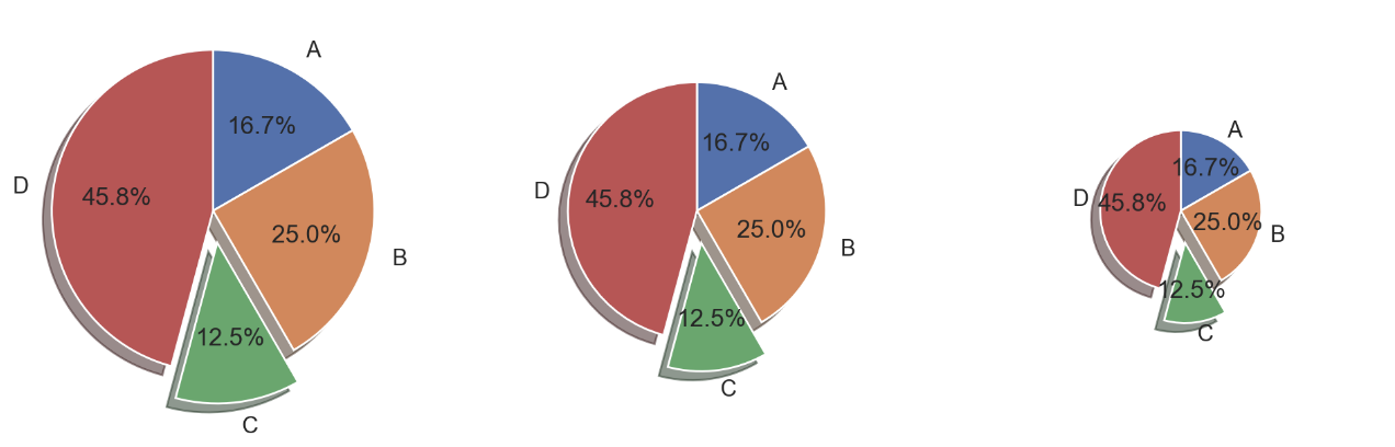
startangle은 시작 각도를 의미하며,explode를 사용하면 특정 label 을 튀어 나오게 하여 강조할 수 있다.shadow를 사용하면 그림자를 추가할 수 있으며autopct는 비율을 작성할 수 있다.labeldistance는 label 을 pie chart 와 얼만큼 떨어져 표시할 것인지를 나타내며,rotatelabels는 label 을 회전한다.counterclock은 시계 방향으로 위치시킬 것인지를 결정할 수 있다. 마지막으로radius는 pie chart 의 크기를 결정한다.
labels = ['A', 'B', 'C', 'D']
data = np.array([60, 90, 45, 165]) # total 360

fig, axes = plt.subplots(1, 3, figsize=(12, 7))
explode = [0, 0, 0.2, 0]

for size, ax in zip([1, 0.8, 0.5], axes):
    ax.pie(data, labels=labels, explode=explode, startangle=90, counterclock=False,
           shadow=True, autopct='%1.1f%%', labeldistance=1.15, radius=size)
plt.show()
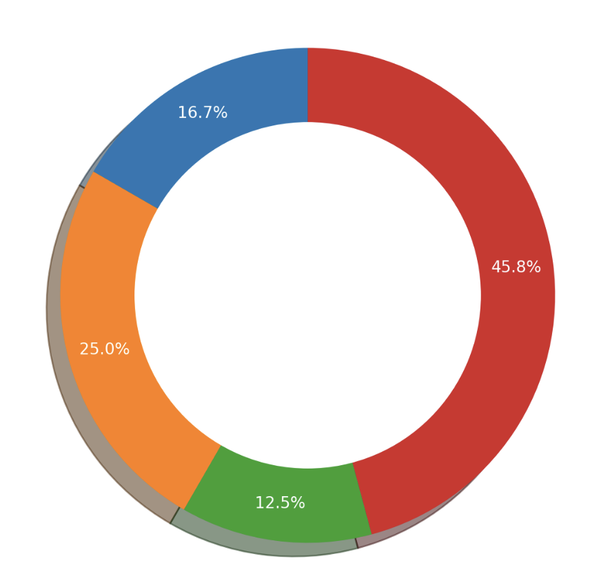
- dount chart 는 pie chart 의 변형으로 자주 사용된다. 중간이 비어있는 pie chart 로서 디자인적으로 선호되는 편이다.
-
인포그래픽에서 종종 사용되며 시각화 라이브러리인
Plotly에서 쉽게 사용이 가능하다.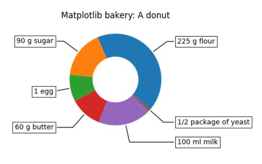
- pie chart 에
plt.Circle을 이용하여.add_artist로 추가해준다.
fig, ax = plt.subplots(1, 1, figsize=(7, 7))


ax.pie(data, labels=labels, startangle=90,
      shadow=True, autopct='%1.1f%%', pctdistance=0.85, textprops={'color':"w"})

# 좌표 0, 0, r=0.7, facecolor='white'
centre_circle = plt.Circle((0,0),0.70,fc='white')
ax.add_artist(centre_circle)

plt.show()
- sunburst chart 는 햇살(sunburst)을 닮은 차트로서, 계층적 데이터를 시각화하는 데 사용된다.
-
구현 난이도에 비해 화려하다는 장점이 있지만, 오히려 Treemap 이 같은 기능을 하여 더 추천된다. 이 또한
Plotly로 쉽게 사용이 가능하다.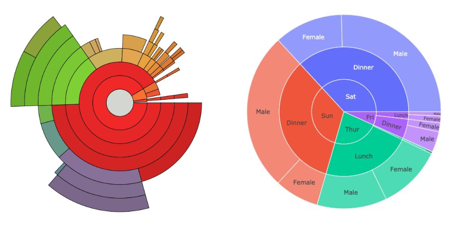
다양한 시각화 라이브러리
- 좀 더 다양한 시각화 라이브러리를 알아보자. 특정 기능에 집중되어 있는 경우가 많다.
Missingno
- Missingno 는 결측치(missing value)를 체크하는 시각화 라이브러리다.
import missingno as msno

msno.matrix(dataset, sort='descending') # 결측치를 matrix 로 나타내어 흰 부분으로 표시한다.
msno.bar(dataset) # 결측치 개수를 직접적으로 bar chart 로 그림
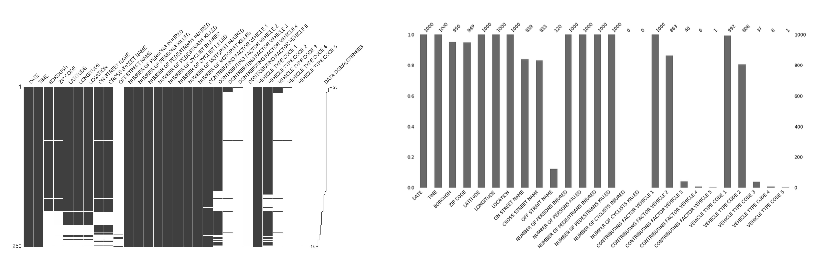
- 그러나 개인적으로
pandas와sns.heatmap을 통하여 확인하는 것도 코드적으로 그렇게 길지 않기 때문에 사용할 일이 별로 없다.
Treemap
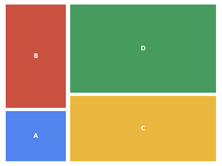
- Treemap 은 계층적 데이터를 직사각형을 사용하여 포함 관계를 표현한 시각화 방법이다. 사각형을 분할하는 타일링 알고리즘에 따라 형태가 다양해지고, 큰 사각형을 분할하여 전체를 나타내는 모자이크 플롯(Mosaic plot)과도 유사하다.
squarify나Plotly의 treemap 을 이용하면 된다.
import squarify

fig, ax = plt.subplots()
values = [100, 200, 300, 400]
label = list('ABCD')
color = ['#4285F4', '#DB4437', '#F4B400', '#0F9D58']

squarify.plot(values, label=label, color=color, pad=0.2,
               text_kwargs={'color':'white', 'weight':'bold'}, ax=ax)

ax.axis('off')
plt.show()
-
Plotly는 사각형 내부에 사각형을 포함시켜 더 계층적인 표현이 가능하다.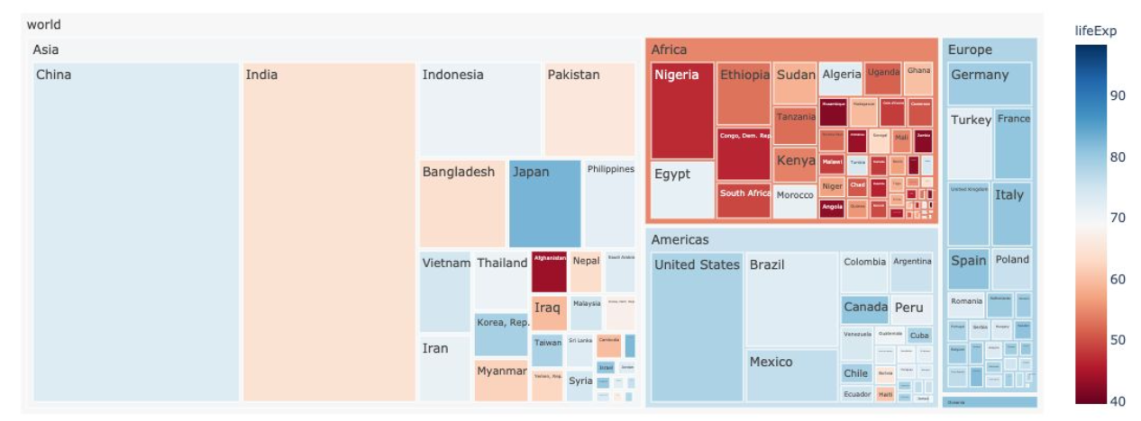
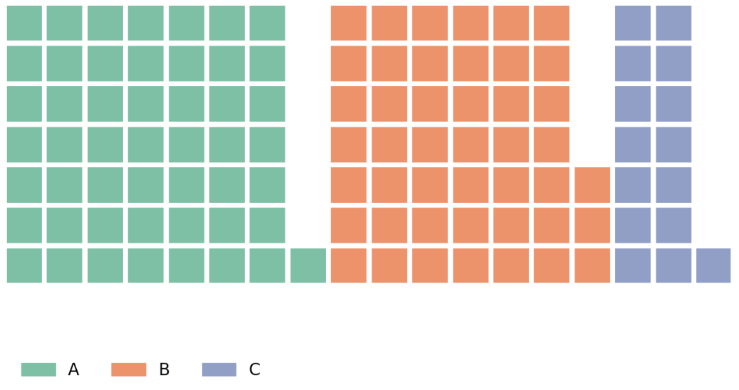
waffle chart
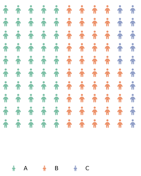
- 와플 형태로 discrete 하게 값을 나타내는 차트다. 기본적인 형태는 정사각형이나 원하는 벡터 이미지로도 사용 가능하다.
- 또한 Icon 을 사용한 Waffle Chart 도 가능하다. Pictogram Chart 라고 불리며, 인포그래픽에서 유용하다.
- 자세한 사용법은 추후 사용할 일이 있을 때 공식문서를 참고하자. 아래는 예제이다.
fig1 = plt.figure(
    FigureClass=Waffle,
    rows=7,
    values=data,
    legend={'loc': 'lower left', 'bbox_to_anchor': (0, -0.4), 'ncol': len(data), 'framealpha': 0},
    block_arranging_style= 'new-line',
)

fig2 = plt.figure(
    FigureClass=Waffle,
    rows=10,
    values=data,
    legend={'loc': 'lower left', 'bbox_to_anchor': (0, -0.4), 'ncol': len(data), 'framealpha': 0},
    icons='child',
    icon_legend=True,
    font_size=15,
)

plt.show()
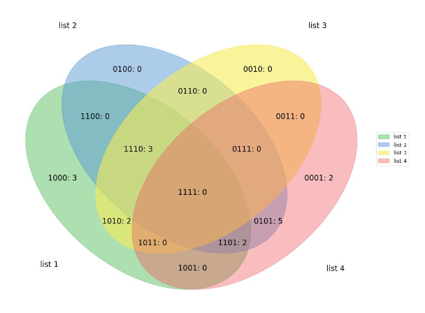
Venn
- 집합(set) 등에서 사용하는 익숙한 벤 다이어그램을 그리는 시각화 라이브러리다.
matplotlib_venn을 사용한다. -
EDA 보다는 출판 및 프레젠테이션에 사용한다. 디테일한 사용이 draw.io 나 ppt 에 비해 어렵기 때문에 잘 사용하지 않는다.
Plotly
- 인터랙티브 시각화에 가장 많이 사용되는 라이브러리가 Plotly 다. Matplotlib 도 인터랙티브를 제공하지만, 주피터 노트북 환경 또는 Local 에서만 실행할 수 있다.
- Plotly 는 Python 뿐 아니라 R, JS 에서도 제공한다. 또한 예시와 문서화가 잘 되어있다.
- 통계 시각화 외에도 지리 시각화, 3D 시각화, 금융 시각화 등 다양한 시각화 기능을 제공한다. Plotly 는 Js 시각화 라이브러리 D3js 를 기반으로 만들어졌기 때문에 웹에서 사용이 가능하다. 특히 형광 Color 가 인상적인 라이브러리다.
-
Plotly 는 seaborn 과 유사하게 만들어 쉬운 문법을 가지고 있다. 커스텀 부분이 다소 부족하지만 다양한 함수를 제공한다.
- 자세한 내용은 공식문서를 확인하자.
TSNE, UMAP
sklearn.manifold의TSNE와umap-learn의UMAP을 가지고 차원 축소 알고리즘을 시각화할 수 있다. t-sne, umap 은 차원 축소 알고리즘 중 neighbour graphs 을 이용하는 방법으로 cluster 를 확인하는데 사용된다.- 이 때 2d 로도 많이 그리지만
Plotly를 사용하여 3d 로도 많이 그린다.
from sklearn.manifold import TSNE
from umap import UMAP
import plotly.express as px

df = px.data.iris()

features = df.loc[:, :'petal_width']

## 2d t-sne
tsne = TSNE(n_components=2, random_state=0)
projections = tsne.fit_transform(features)

fig = px.scatter( projections, x=0, y=1, color=df.species, labels={'color': 'species'})

## 3d-tsne
tsne = TSNE(n_components=3, random_state=0)
projections = tsne.fit_transform(features, )

fig = px.scatter_3d(projections, x=0, y=1, z=2, color=df.species, labels={'color': 'species'})
fig.update_traces(marker_size=8)
fig.show()

## 2d-umap
umap_2d = UMAP(n_components=2, init='random', random_state=0)
proj_2d = umap_2d.fit_transform(features)

fig_2d = px.scatter(proj_2d, x=0, y=1, color=df.species, labels={'color': 'species'})
fig_2d.show()

## 3d-umap
umap_3d = UMAP(n_components=3, init='random', random_state=0)
proj_3d = umap_3d.fit_transform(features)

fig_3d = px.scatter_3d(proj_3d, x=0, y=1, z=2, color=df.species, labels={'color': 'species'})
fig_3d.update_traces(marker_size=5)
fig_3d.show()
Reference
- Naver Connect BoostCamp 강의
- https://matplotlib.org/stable/index.html
- https://seaborn.pydata.org/
댓글 남기기