
[Pytorch, Trouble Shooting] Array/Tensor, Indexing & Slicing, Axis, Shape
앞선 포스트에서 Pytorch 가 무엇인지 알아보고, tensor 의 생성 그리고 tensor 의 index 및 shape(rank) 조작을 간단히 살펴봤다.
다차원 배열(행렬) 연산은 딥러닝에서 가장 필수적인 연산이다. numpy 와 torch 는 이러한 다차원 배열 연산을 지원하는 라이브러리로 매우 잘 호환된다. 그러나 numpy 는 일반적인 ML 을 위해 사용되고, torch 는 torch.Tensor 를 통해 무거운 행렬 연산에 최적화되어 GPU 사용을 지원한다. 따라서 딥러닝 과정에서 torch 의 사용은 매우 일반적이다.
이 포스트에서는 numpy 와 torch 를 사용하여 모델링을 하거나 전처리, 학습을 구현하면서 수없이 사용되는 배열 또는 행렬의 indexing, slicing, axis(dim) 에 대해 정리하고자 한다. 이를 위해서 numpy 공식문서 를 활용하여 정리한다. 이를 알면 torch 에서 사용되는 indexing, slicing, axis 또한 쉽게 이해할 수 있기 때문이다. 추가로 정리하다가 두 라이브러리 사이의 차이가 존재하면 언급할 것이다.
Array & Tensor
- numpy 의 핵심에는
ndarray객체가 있다. 이는 동일한 데이터 타입의 $n$ 차원 배열을 캡슐화 한 것이며, 이를 활용한 많은 연산은 성능을 위해 컴파일된 코드로 실행된다. - numpy ndarray 배열과 python 의 sequence 자료형(List, Tuple 등) 간에는 몇 가지 중요한 차이점이 있다.
- numpy 배열은 생성 시 크기가 고정되며, python list 처럼 동적으로 크기가 변하지 않는다. 즉 ndarray 의 크기를 변경하면 새로운 배열이 생성되고 원래 배열은 삭제된다.
- 또한 numpy 배열의 요소는 python list 와 달리 모두 동일한 데이터 타입이어야 하며, 따라서 메모리에서 동일한 크기를 가진다.
- 이러한 numpy ndarray 는 대규모 데이터에 대해 복잡한 수학적 연산을 쉽게 수행할 수 있도록 한다. 또한 일반적으로 python 의 내장 sequence 를 사용하는 것보다 더 효율적으로, 더 적은 코드로 실행된다.
- 점점 더 많은 과학 및 수학 기반 python 패키지들이 numpy 배열을 사용하고 있다. 이러한 패키지들은 python sequence 입력을 지원하지만, 처리 전에 이를 numpy 배열로 변환하고 numpy 배열을 출력한다.
- 이는 pytorch 도 마찬가지다. 물론 pytorch 는 numpy 기반 배열을 사용하지 않고, 자체적인 tensor 객체인
torch.Tensor를 사용한다. - 그러나 torch 의 tensor 객체와 numpy 의 ndarray 객체는 매우 유사하며, 많은 면에서
torch.Tensor와np.ndarray는 호환된다. - 따라서 오늘날의 과학/수학 기반의 python 소프트웨어를 효율적으로 사용하려면 python 내장 시퀀스 타입만 아는 것으로는 충분하지 않고, numpy 배열의 사용법도 알아야한다.
tensor
- tensor 란 수학적인 개념으로 데이터의 배열이라고 볼 수 있다. 이 배열은 여러 차원을 가질 수 있기 때문에 다차원 배열이라고 정의되기도 한다.
- 컴퓨터로 구현되는 딥러닝 모델은 문자열, 이미지, 오디오에 대해 알지 못한다. 따라서 모델은 입력 tensor 에서 구조와 패턴을 찾아내고, 출력 tensor 와의 관계를 인식하기 위해 숫자로 표현된 데이터를 다룬다.
-
Computer Vision 에서 사용하는 데이터는 image 다. 여기서 마찬가지로 데이터는 숫자로 변환될 수 있는 모든 것을 의미한다.
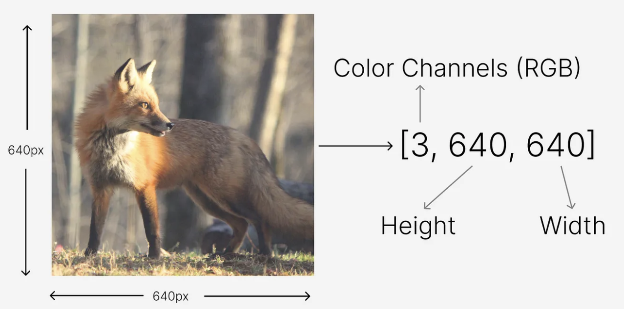
- 그렇다면 image 를 하나의 tensor 로 변환할 수 있다. 즉 위 그림처럼 640 x 640 크기의 이미지를 tensor 로 변환할 수 있다.
- 이 때 tensor 의 모양은
[3, 640, 640]이 되는데, 여기서 3 은 image 에서의 색상 채널 RGB 를 나타내고, 640 은 각각 이미지의 높이와 너비를 의미한다. - 이러한 tensor 는 딥러닝 모델의 가장 기본이다. 왜냐하면 neural network 는 입력 및 출력의 데이터 구조로 tensor 를 사용하기 때문이다.
-
또한 tensor 는 차원/랭크(Dimension/Rank), 모양(Shape), 그리고 데이터 타입(DType) 이라는 특별한 특성을 가지고 있다.
차원/랭크(Dimension/Rank)
- dimension, 또는 tensor 에서 rank 라고도 불리는 것은 tensor 가 가진 차원의 수를 의미한다.
-
tensor 의 차원을 알기 위해서는 아래 그림과 같이 왼쪽에서 시작하여 배열이 아닌 요소에 도달할 때까지
[의 수를 세면 된다. 이는 numpy ndarray 도 마찬가지다.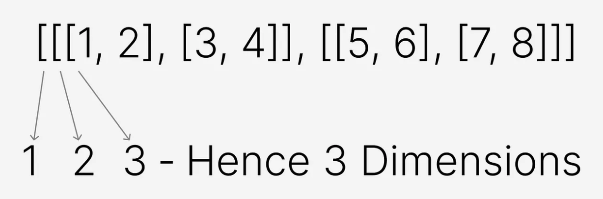 3 차원의 배열, 즉 tensor
 - tensor 는 배열의 특수한 형태이지만, rank 에 따라 특정 이름으로 불린다.
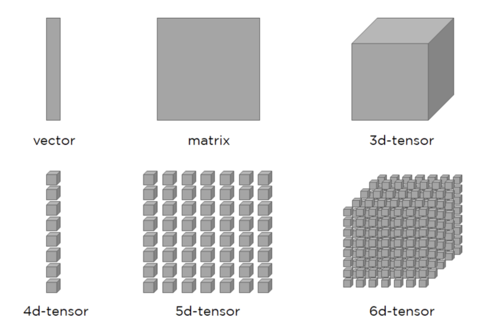
- rank 0: rank 가 0 인 tensor 를 scalar 라고 부른다. 이는 실수 또는 상수와 같은 단일 값을 나타낸다.
- rank 1: rank 가 1 인 tensor 를 vector 라고 부른다. vector 는 1차원 데이터를 가지며, 값의 목록으로 표현할 수 있다.
- rank 2: rank 가 2 인 tensor 를 matrix 라고 부른다. matrix 는 2차원 데이터를 가지며, 이미지나 표 형식 데이터를 나타내는 데 사용된다.
- rank 3: rank 가 3인 tensor 는 3D tensor 라고 부른다. 이는 큐브 또는 matrix 의 스택으로 시각화할 수 있다.
- rank 4: rank 가 4인 tensor 는 4D tensor 라고 부른다. 딥러닝에서 4D tensor 는 batch 형태의 이미지를 나타내며, 네 번째 차원이 batch 의 크기를 나타낸다.
- 또한 tensor 는 문제와 데이터의 복잡성에 따라 더 높은 rank 를 가질 수도 있다.
- 예를 들어, 비디오 데이터는 5D tensor 라고 볼 수 있는데, 이때 각 요소는 비디오의 한 프레임을 나타내는 4D tensor 를 포함한다.
-
또 한가지 유념할 것은, torch 에서는 channel 이 첫번째 차원에 나오게 되고, batch 형태에서는 batch size 가 맨 처음 나오게 된다. 즉, image 를 대상으로 했을 때 아래와 같다.
\[(B, C, H, W)\] -
아래 그림은 rank 별 tensor 를 나타낸 것이다.
모양(Shape)
- tensor 의 shape 은 dimension(rank)과 관련이 있다. shape 는 각 차원의 길이를 나타내는 숫자 배열이다.
-
tensor 의 shape 을 식별하는 방법은 각 차원에서의 요소 수를 알아내는 것이다.
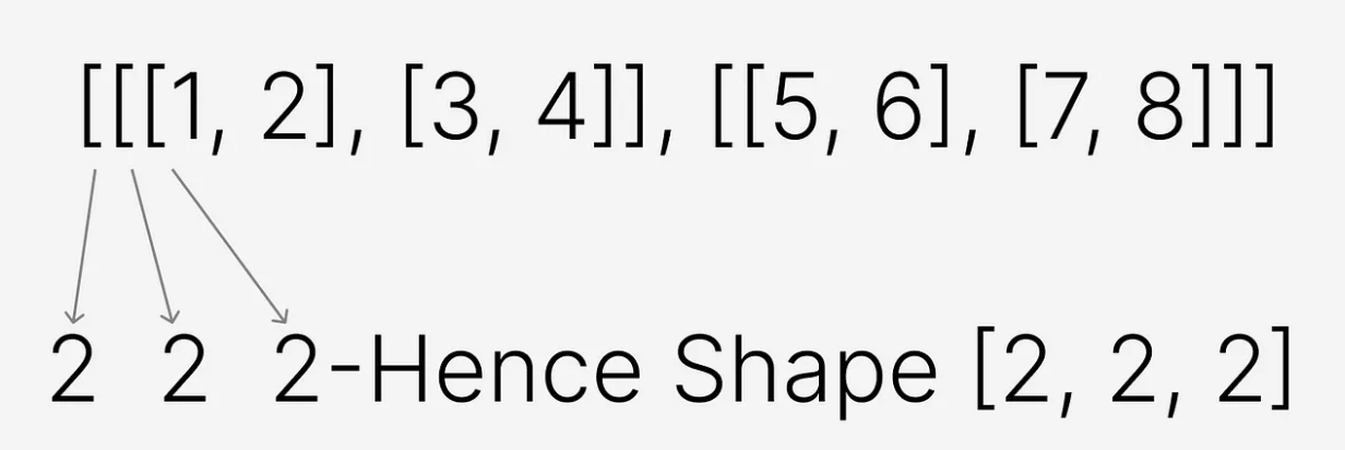
- 위의 예시에서 tensor 는 3 개의 차원을 가지고 있고, 각 차원에 두 개의 요소를 가지고 있다.
- 따라서 tensor 의 shape 은
[2, 2, 2]가 된다. 이 때 요소가 배열이든 값이든 관계없이 둘 다 요소로 간주된다. - 딥러닝에서 겪는 문제 중 대부분은 shape 의 불일치와 관련이 있다.
- 예를 들어 특정 shape 을 입력으로 받거나 출력하도록 학습된 모델에 다른 shape 의 tensor 를 전달할 수 없다.
- 따라서 모델이 기대하는 정확한 shape 으로 tensor 를 준비해야 하기 때문에 중요한 주제다.
데이터 타입(DType)
- tensor 의 데이터 타입은 tensor 가 저장할 수 있는 값의 타입을 정의한다.
- 예를 들어 정수(integers), 부동소수점(floating-point), 참/거짓(booleans) 등의 데이터 타입이 있다.
- 부동소수점(floating-point)이란 컴퓨터가 소수점이 포함된 실수를 표현하기 위한 방법 중 하나로, 고정소수점과 달리 소수점이 고정되어 있지 않고 좌우로 움직일 수 있다. 따라서 표현할 수 있는 수의 범위가 매우 넓다는 장점이 있다.
- 일반적인 데이터 타입으로는
int32,float32,bool등이 있으며, 데이터 타입은 요소를 저장하는 데 필요한 정밀도와 메모리 요구 사항을 결정한다. - 데이터 타입에 적혀있는 숫자는
bit를 뜻하며 일반적으로8, 16, 32, 64가 있다. 숫자가 작을수록 메모리 사용량이 적고 정밀도가 낮다. 반대로 숫자가 클수록 정밀도가 높지만 메모리 사용량과 연산 비용이 크다. - torch 에는 다양한 데이터 타입이 있는데, torch 의 공식문서에서 모두 확인할 수 있다.
- 기억하면 좋을 것은 torch 를 사용한 딥러닝 모델은 기본 데이터 타입으로
float32타입을 가진다. - 또한
uint8은 8 bit 의 부호 없는 정수로서 image 데이터의 default 값이다.opencv등의 라이브러리를 통해서 image normalize 등을 한다면 연산의 결과값 범위가 제한되기 때문에float32나float64로 바꿔줘야 한다. - 추가적으로
float64는double과 같고,int64는long과 같다. - 데이터 타입을 변경할 때는 torch 에서는
torch.Tensor.to()나torch.Tensor.type()를 사용하고, numpy 에서는np.ndarray.astype()을 사용하면 된다.
import numpy as np
import torch

python_array = [[1,2],[3,4]]

n_array = np.array(python_array)
t_tensor = torch.tensor(python_array)

print(type(n_array), n_array.dtype)        # <class 'numpy.ndarray'> int64
print(type(t_tensor), t_tensor.dtype)      # <class 'torch.Tensor'> torch.int64

n_array_f = n_array.astype(np.float32)
t_tensor_f = t_tensor.to(torch.float32)

print(type(n_array_f), n_array_f.dtype)    # <class 'numpy.ndarray'> float32
print(type(t_tensor_f), t_tensor_f.dtype)  # <class 'torch.Tensor'> torch.float32
ndarray vs. tensor
- torch 의
torch.Tensor객체는 GPU 연산을 지원하며, 자동 미분(autograd) 기능을 제공하는 등 딥러닝을 위한 기능이 추가된 객체다. - 반면 numpy 의
np.ndarray는 기본적으로 CPU 에서만 동작하고, 자동 미분 같은 기능은 제공하지 않는다. - 그러나
torch.Tensor를np.ndarray로 변환하거나, 그 반대로 변환하는 것은 매우 간단하다. 이를 통해 두 라이브러리 간의 상호 운용성이 뛰어나다.torch.from_numpy()를 사용해np.ndarray를torch.Tensor로 변환할 수 있다..numpy()메서드를 사용해torch.Tensor를np.ndarray로 변환할 수 있다.- 따라서 GPU 를 사용하여 빠르게 학습하려는 경우 numpy 에서 torch 로 변환한다.
- 또한 torch 의 tensor 연산은 numpy 의 배열 연산과 매우 유사한 API 를 제공하고 있다. 예를 들어, 배열 간의 산술 연산이나 브로드캐스팅, indexing 등은 거의 동일한 방식으로 동작한다. 이 때문에 numpy 를 잘 조작할 수 있다면 torch 도 다루기 어렵지 않다.
- 그러나 tensor 의 shpae 을 조작하는 측면에서 numpy 와 torch 에 다른 점이 있으며, torch 에는 tensor 의 shape 를 조작하는 다양한 메서드를 제공한다. 이는 아래에서 보도록 하자.
torch.Tensor vs torch.tensor
- torch 공식문서에 보면
torch.Tensor와torch.tensor가 모두 존재한다. 이 두 개의 차이점은 뭘까? torch.Tensor는 Tensor 자료구조 클래스다. 즉torch.Tensor()를 통해 인스턴스를 생성할 수 있다.- 반면
torch.tensor는 어떤 data 를torch.Tensor로 copy 해주는 메서드다. 이 때 주어진 data 가torch.Tensor클래스가 아니면 적용하여 복사한다.
Array/Tensor 생성
- numpy 와 torch 에서는 tensor 를 생성하는 다양한 방법이 있다. 특히 원하는 범위 내의 숫자들로만 이루어진 tensor 를 만들수도 있고, 랜덤하게 숫자를 가지는 tensor 를 만들수도 있다.
- 각 메서드의 argument 나 출력은 주석을 통해 표시한다.
numpy
- python list 를 입력으로 주어
np.ndarray를 만들 수 있다.
import numpy as np

python_list = [[1, 2], [3, 4]]
n_array = np.array(python_list)

print(n_array)        # [[1 2], [3 4]]
print(type(n_array))  # <class 'numpy.ndarray'>
print(n_array.shape)  # (2, 2)
print(n_array.size)   # 4
print(n_array.dtype)  # int64
- 위에서 shape 은 tensor 의 모양, size 는 배열의 크기를 뜻한다.
- 이 때
np.array()안에 dtype 을 지정해줄 수도 있다.
import numpy as np

python_list = [[1, 2], [3, 4]]
n_array = np.array(python_list, dtype=np.float32)

print(n_array)        # [[1. 2.], [3. 4.]]
print(type(n_array))  # <class 'numpy.ndarray'>
print(n_array.shape)  # (2, 2)
print(n_array.size)   # 4
print(n_array.dtype)  # float32
np.arange()를 통하여 1D array 를 만들 수 있다. argument 에 주의하자.
import numpy as np

n_array = np.arange(10) # stop
print(n_array)   # [0 1 2 3 4 5 6 7 8 9]

n_array2 = np.arange(2, 10, dtype=np.float32) # start, stop, dtype
print(n_array2)  # [2. 3. 4. 5. 6. 7. 8. 9.]

n_array3 = np.arange(2, 3, 0.1) # start, stop, step
print(n_array3)  # [2. 2.1 2.2 2.3 2.4 2.5 2.6 2.7 2.8 2.9]
np.linspace()또한 1D array 를 만들 수 있다. 이 때 start 와 stop 사이를 일정한 길이로 잘라 argument 로 주어진 요소의 개수를 맞춘다.
import numpy as np

n_array = np.linspace(1., 4., 6) # start, stop, num
print(n_array)  # [1.  1.6 2.2 2.8 3.4 4. ]
- 이 함수는
np.arange()와 달리 stop 또한 값으로 포함할 수 있으며 배열의 길이를 결정할 수 있다는 장점이 있다. np.eye(),np.diag()는 2D array 를 만드는데 사용된다.np.eye()는 항등행렬(identity matrix)을 만들 때 사용한다. 이 때 정방행렬이 아니어도 상관없이 row 와 column index 가 같은 $i = j$ 인 부분을 1 로, 나머지는 0 으로 만든다.
import numpy as np

print(np.eye(3))
# [[1. 0. 0.]
#  [0. 1. 0.]
#  [0. 0. 1.]]

print(np.eye(3, 5))
# [[1. 0. 0. 0. 0.]
#  [0. 1. 0. 0. 0.]
#  [0. 0. 1. 0. 0.]]
np.diag(v, k=0)는 대각행렬을 만들 때 사용한다. 이 때v가 1D array 이면k번째부터v의 원소로 대각을 구성하며, 2D array 이면 해당v의k번째부터 대각 요소를 출력한다.
import numpy as np

np.diag([1, 2, 3])
# [[1 0 0]
#  [0 2 0]
#  [0 0 3]]

np.diag([1, 2, 3], 1)
# [[0 1 0 0]
#  [0 0 2 0]
#  [0 0 0 3]
#  [0 0 0 0]]

a = np.array([[1, 2], [3, 4]])
np.diag(a)
# [1 4]
- 이외에 일반적인 3D array 를 만들 수 있는 함수도 있다.
np.zeros(shape, dtype)은 0 으로 이루어진shape크기의 tensor 를 만들어낸다. 반면np.ones(shape, dtype)은 1 로 이루어진shape크기의 tensor 를 만들어낸다. 물론 두 함수 모두 vector 를 만들어낼 수도 있다.
import numpy as np
print(np.zeros(2))  # [0. 0.]
print(np.zeros((2, 3)))
# [[0. 0. 0.]
#  [0. 0. 0.]]
print(np.zeros((2, 3, 2)))
# [[[0. 0.]
#   [0. 0.]
#   [0. 0.]]
#  [[0. 0.]
#   [0. 0.]
#   [0. 0.]]]

print(np.ones(2))  # [1. 1.]
print(np.ones((2, 3)))
# [[1. 1. 1.]
#  [1. 1. 1.]]
print(np.ones((2, 3, 2)))
# [[[1. 1.]
#   [1. 1.]
#   [1. 1.]]
#  [[1. 1.]
#   [1. 1.]
#   [1. 1.]]]
- 이외에
np.random에서는 주어진 범위에서 랜덤으로 정수를 가지는 tensor 와 normal 분포에서 랜덤으로 샘플링한 요소를 가지는 tensor 를 만들 수 있다. 각각np.random.randint(low, high, size)와np.random.normal(loc, scale, size)이다. 또한np.random.uniform(low, high, size)로 균등분포에서 샘플링할 수도 있다.
import numpy as np

print(np.random.randint(0,10,(3,3)))
# [[4 9 0]
#  [2 9 5]
#  [1 1 9]]
print(np.random.normal(0, 1, (3,3)))
# [[-0.75426693  0.38773244 -0.6050126 ]
#  [-0.61388604 -1.29974758 -0.39227839]
#  [ 0.38090377  0.13244095 -0.74426853]]
print(np.random.uniform(0, 10,(3,3)))
# [[5.56288317 8.11895323 0.97697638]
#  [8.20726984 6.71551445 8.95123704]
#  [5.73262824 8.6680865  2.54221576]]
torch
- python list 입력으로 주어
torch.Tensor를 만들 수 있다. 마찬가지로 데이터 타입을 줄 수 있다.
import numpy as np

python_list = [[1, 2], [3, 4]]
t_tensor = torch.tensor(python_list, dtype=torch.float32)

print(t_tensor)        # tensor([[1., 2.], [3., 4.]])
print(type(t_tensor))  # <class 'torch.Tensor'>
print(t_tensor.shape)  # torch.Size([2, 2])
print(t_tensor.size()) # torch.Size([2, 2])
print(t_tensor.dtype)  # torch.float32
torch.from_numpy()를 통해 numpy 배열을torch.Tensor로 만들 수 있다.
import numpy as np
import torch

n_array = np.arange(5)
t_tensor = torch.from_numpy(n_array)
print(t_tensor)        # tensor([0, 1, 2, 3, 4])
print(t_tensor.dtype)  # torch.int64
print(t_tensor.type()) # torch.LongTensor
print(type(t_tensor))  # <class 'torch.Tensor'>
torch.as_tensor()는 list 혹은 numpy 배열을torch.Tensor로 만들 수 있다.
import numpy as np
import torch

p_list = [1,2,3,4,5]
t_tensor1 = torch.as_tensor(p_list)
print(t_tensor1)           # tensor([1, 2, 3, 4, 5])
print(t_tensor1.dtype)     # torch.int64
print(t_tensor1.type())    # torch.LongTensor
print(type(t_tensor1))     # <class 'torch.Tensor'>

n_array = np.arange(1, 6)
t_tensor2 = torch.as_tensor(n_array)

print(t_tensor2)           # tensor([1, 2, 3, 4, 5])
print(t_tensor2.dtype)     # torch.int64
print(t_tensor2.type())    # torch.LongTensor
print(type(t_tensor2))     # <class 'torch.Tensor'>
- 여기서 중요한 것은
torch.from_numpy()와torch.as_tensor()를 사용해서 만든torch.Tensor는 numpy 배열과 같은 메모리 주소를 참조한다. 즉 shallow copy 와 유사한 sharing 이 일어난다. 이에 따라 numpy 배열을 수정하면torch.Tensor도 수정된다. - 반면에
torch.tensor()는 deep copy 가 되어 원본가 완전히 독립적인 객체가 된다.
import numpy as np
import torch

p_list = [[1,2],[3,4],[5,6]]
n_array = np.array(p_list)
t_tensor1 = torch.from_numpy(n_array)
print(t_tensor1)
# tensor([[1, 2],
#         [3, 4],
#         [5, 6]])
n_array[0][0] = 100
print(t_tensor1)
# tensor([[100, 2],
#         [3, 4],
#         [5, 6]])
n_array = np.array(p_list)
t_tensor2 = torch.as_tensor(n_array)
print(t_tensor2)
# tensor([[1, 2],
#         [3, 4],
#         [5, 6]])
n_array[0][0] = 100
print(t_tensor2)
# tensor([[100, 2],
#         [3, 4],
#         [5, 6]])
n_array = np.array(p_list)
t_tensor3 = torch.tensor(n_array)
print(t_tensor3)
# tensor([[1, 2],
#         [3, 4],
#         [5, 6]])
n_array[0][0] = 100
print(t_tensor3)
# tensor([[1, 2],
#         [3, 4],
#         [5, 6]])
torch.arange(start, end, step)을 통해 1D tensor 를 만들 수 있다.
import torch

t_tensor = torch.arange(1, 10, 2, dtype=torch.float32)
print(t_tensor)   # tensor([1., 3., 5., 7., 9.])
torch.ones(size),torch.zeros(size)는 각각 1 과 0 으로만 이루어진 tensor 를 원하는 shape(size) 에 맞게 생성할 수 있다.
import torch

one_tensor = torch.ones((2, 3))
print(one_tensor)
# tensor([[1., 1., 1.],
#         [1., 1., 1.]])
zero_tensor = torch.zeros((3, 2))
print(zero_tensor)
# tensor([[0., 0.],
#         [0., 0.],
#         [0., 0.]])
torch.ones_like(input)와torch.zeros_like(input)은 input 의 shape 과 같은 1 과 0 으로만 이루어진 tensor 를 반환한다.
import torch

one_tensor = torch.ones((2, 3))
from_one_to_zero = torch.zeros_like(one_tensor)
print(from_one_to_zero)
# tensor([[0., 0., 0.],
#         [0., 0., 0.]])
zero_tensor = torch.zeros((3, 2))
from_zero_to_one = torch.ones_like(zero_tensor)
print(from_zero_to_one)
# tensor([[1., 1.],
#         [1., 1.],
#         [1., 1.]])
torch.randint(low=0, high, size)는 [low, high) 범위의 정수를 랜덤하게 샘플링하여 shape(size)에 맞게 생성한다.
import torch

t_tensor = torch.randint(1, 9, (2, 4))
print(t_tensor)
# tensor([[8, 8, 2, 5],
#         [4, 1, 7, 6]])
torch.rand(size)와torch.randn(size)는 각각 [0, 1) 범위의 uniform distribution 에서 랜덤으로 샘플링한 tensor 와 $N \sim (0, 1)$ 인 gaussian distribution 에서 랜덤으로 샘플링한 tensor 를 생성한다.
import torch

uni_tensor = torch.rand((2, 4))
print(uni_tensor)
# tensor([[0.3056, 0.3277, 0.0654, 0.9210],
#         [0.1507, 0.6506, 0.6631, 0.3949]])

normal_tensor = torch.randn((3, 2))
print(normal_tensor)
# tensor([[-0.3928, -0.3684],
#         [ 3.0273,  1.2370],
#         [-0.2499,  0.3665]])
Indexing & Slicing
- indexing 과 slicing 은 tensor 내 원하는 위치의 원소 부분집합을 가져오는 방법이다.
- PyTorch 로 딥러닝을 할 때 input 으로 사용하는 데이테셋이 다차원의 행렬인 tensor 이기 때문에, indexing 과 slicing 은 자주 사용하게 된다.
- 이는 tensor 의 차원이 많아질수록 헷갈리는 개념이기 때문에 정확하게 이해하고 있어야 한다.
- 마찬가지로
numpy의 indexing 과 slicing 을 잘 알고 있으면torch의 indexing 과 slicing 도 어렵지 않게 이해할 수 있다. - 앞으로 예제에서는 아래의 tensor 들을 사용하도록 하자.
import numpy as np
import torch

p_list = [[0,1,2,3],
          [4,5,6,7],
          [8,9,10,11]]
n_array = np.array(p_list)
t_tensor = torch.tensor(p_list)
Single element indexing
- python 의 list indexing 과 똑같은 방식으로 사용할 수 있다. 예제가
(3, 4)의 shape 을 가지고 있기 때문에 하나의 index 로 indexing 하면 맨 앞의 차원에서 해당 index 를 가져오고 나머지 차원은:이 된다. - 예를 들어 두 개의 index
(i, j)를 사용하면 가장 바깥 차원의i번째 원소를 가져오고, 그 가져온 원소에서j번째 원소를 가져온다. :는 해당 차원 전체를 가져온다는 것을 의미한다.- 그리고 모든 index 는 zero-base $0 \leq n_i < d_i$ 로 0 부터 시작하며, $n_i < 0$ 인 경우 해당 index 는 $n_i + d_i$ 다.
print(n_array[0])      # [0 1 2 3]
print(n_array[0, :])   # [0 1 2 3]
print(t_tensor[-1])    # tensor([ 8,  9, 10, 11])
print(t_tensor[-1, :]) # tensor([ 8,  9, 10, 11])

print(n_array[0][1])   # 1
print(n_array[0, 1])   # 1
print(t_tensor[0][1])  # tensor(1)
print(t_tensor[0, 1])  # tensor(1)
- 만약 tensor 가 3 차원 이상의 shape
(r, k, i, j)가 있다고 해보자. - 이 경우 indexing 을 위한 index 를 차원의 개수 4 개만큼 사용할 수 있고, 사용된 index 는
r부터 해당되고 이후 index 는 차례대로 다음 차원에 해당된다. - 아래 예제를 보자.
tensor_3d = torch.randint(0, 9, (2, 3, 4, 5))

print(tensor_3d[0, 1, :, 3])
# r 차원에서 0 번째 요소 -> shape : (3, 4, 5)
# 해당 tensor 의 k 차원에서 1 번째 요소 -> shape : (4, 5)
# 해당 tensor 의 i 차원에서 전체(:) 요소 -> shape : (4, 5)
# 해당 tensor 의 j 차원에서 3 번째 요소 -> shape : (4)

# tensor([8, 7, 6, 6])

print(tensor_3d[0, 1, :, 3].shape)
# tensor.Size([4])
- 만약 CNN 에서 shape 이
(32, 3, 24, 24)인 32 batch size 의 24 x 24 image tensor 가 있을 때, 모든 batch 에서 각 image 의 0 번째 채널만 가지고 오고 싶다면[:, 0, :, :]로 indexing 하면 된다. - 주의할 점은 하나의 indexing
[ ]안에서,로 연결되는 것과[][]로 나눠서 indexing 하는 것이 결과가 다른 경우가 있다.
print(n_array[:, -1])   # [ 3  7 11]
print(n_array[:][-1])   # [ 8  9 10 11]
print(t_tensor[:, -1])  # tensor([ 3,  7, 11])
print(t_tensor[:][-1])  # tensor([ 8,  9, 10, 11])
- 이는
[:, -1]의 경우 전체를 가져오고 그 다음 차원의-1요소를 가져오는 반면,[:][-1]은 전체를 그대로 가져오고 그 다음 차원이 아닌 가장 바깥 차원의-1번째 요소를 가져오기 때문이다. - 따라서 하나의 indexing 으로 엮어줘야 차원을 순차적으로 흘러가며 indexing 해올 수 있다.
- 그리고 당연하게 indexing 의 출력은 원본의 tensor 와 독립적인 것이 아니라 메모리 주소를 공유한다. 따라서 python 처럼 indexing 에 새로운 값을 할당하면 원본 tensor 도 해당 위치의 값이 바뀐다.
Slicing
- slicing 은
start:stop:step로 원하는 구간에서 값을 가져올 수 있다. 이 때 하나의 slicing 단위는 indexing 에서와 마찬가지로 대응되는 차원에서만 수행된다. start는 생략되면 0 이며,stop은 생략되면 맨 마지막 요소까지다.step은 0 이 될 수 없고, 음수의 경우 순서가 거꾸로 진행된다.- 그러나
torch에서는 slicing 에서step에 음수가 들어갈 수 없다. 이에 따라 특정 tensor 의 차원을 뒤집을 때는flip(dims)함수를 이용한다.
print(n_array[:1])           # [[0 1 2 3]]
print(n_array[:1, 1:])       # [[1 2 3]]
print(n_array[:1,1::2])      # [[1 3]]
print(n_array[:1,1::-1])     # [[1 0]]
print(t_tensor[:1])          # tensor([[0, 1, 2, 3]])
print(t_tensor[:1, 1:])      # tensor([[1, 2, 3]])
print(t_tensor[:1,1::2])     # tensor([[1, 3]])
print(t_tensor[:1,:2])       # tensor([[0, 1]])
print(t_tensor[:1,:2].flip(0))
# tensor([[0, 1]])
print(t_tensor[:1,:2].flip(1))
# tensor([[1, 0]])
Dimensional indexing
numpy와torch에는 shape 를 맞추면서 tensor 를 indexing 과 slicing 을 편하게 할 수 있는 도구들이 있다.Ellipsis와np.newaxis,None이다.- 이는 3 차원 이상의 tensor 에서 indexing 과 slicing 한 후에 해당 tensor 를 연산할 때 shape 을 맞추기 복잡할 수 있는데, 이 때 사용될 수 있다.
Ellipsis는:와 같은 역할을 하는데, 여러 개의:를 하나의Ellipsis로 대체할 수 있다. 그러나 하나의 indexing 에서Ellipsis는 하나만 존재해야 한다.
import numpy as np
import torch

n_array_3d = np.arange(24).reshape(2, 3, 4)
t_tensor_3d = torch.arange(24).reshape(2, 3, 4)

print(n_array_3d[..., 2].shape)   # (2, 3)
print(n_array_3d[:, :, 2].shape)  # (2, 3)

print(t_tensor_3d[..., 2].shape)  # torch.Size([2, 3])
print(t_tensor_3d[:, :, 2].shape) # torch.Size([2, 3])
- indexing 에서
np.newaxis와None는 위치한 곳에 해당하는 차원을 새로 늘려서 1 로 만들어준다. - 그러나
torch에서는np,newaxis를 쓸 수는 없고, 원하는 차원을 새로 만들기 위해서None이나torch.unsqueeze(dim)혹은torch.unsqueeze_(dim)을 사용한다. - 이 때
torch.unsqueeze_(dim)는torch.unsqueeze(dim)와 달리 in-place 로 동작한다. 즉 새로 할당할 필요 없다.
n_array_3d = np.arange(24).reshape(2, 3, 4)
t_tensor_3d = torch.arange(24).reshape(2, 3, 4)

print(n_array_3d.shape)  # (2, 3, 4)
print(n_array_3d[:, np.newaxis, :, :].shape) # (2, 1, 3, 4)
print(n_array_3d[:, None, :, :].shape)       # (2, 1, 3, 4)

print(t_tensor_3d.shape)  # torch.Size([2, 3, 4])
print(t_tensor_3d[:, None, :, :].shape) # torch.Size([2, 1, 3, 4])
print(t_tensor_3d.unsqueeze(1).shape)   # torch.Size([2, 1, 3, 4])
print(t_tensor_3d.unsqueeze_(1).shape)  # torch.Size([2, 1, 3, 4])
Integer array indexing
- 정수로 이루어진 tensor 로 indexing 이 가능하다. 이 때 indexing 에 사용된 tensor 의 각 수는 해당 차원에서 요소들의 index 에 해당한다.
n = np.arange(10, 1, -1)
t = torch.arange(10, 1, -1)

print(n) # [10  9  8  7  6  5  4  3  2]
print(n[np.array([3, 3, 1, 8])]) # [7 7 9 2]
print(n[np.array([3, 3, -3, 8])]) # [7 7 4 2]

print(t) # tensor([10,  9,  8,  7,  6,  5,  4,  3,  2])
print(t[torch.tensor([3, 3, 1, 8])]) # tensor([7, 7, 9, 2])
print(t[torch.tensor([3, 3, -3, 8])]) # tensor([7, 7, 4, 2])
- 또한 원본 tensor 의 차원의 수만큼 다차원의 integer array 도 사용 가능하다. 이 때 해당 array index 는 그 위치의 차원에 적용되고, array index 가 원본 tensor 의 각 차원에 모두 존재한다면, 출력의 차원은 array index 의 차원과 같다. 주의할 점은 integer array 들의 요소의 개수가 같아야 한다.
x[[0, 2, 4], [0, 1, 2]]인 경우 출력은[x[0, 0], x[2, 1], x[4, 2]]가 된다.- 아래 예시를 보자.
n = np.arange(35).reshape(5, 7)
t = torch.arange(35).reshape(5, 7)

print(n[[0,1], [2,3]])  # [2, 10]
print(t[[0,1], [2,3]])  # tensor([2, 10])

n = np.arange(24).reshape(2, 3, 4)
t = torch.arange(24).reshape(2, 3, 4)

print(n[[0,1], [0,1]])
# [[ 0  1  2  3]
#  [16 17 18 19]]
print(n[[0,1], [0,1], [1,1]])  # [1, 17]
print(n[[[0,1], [0,1]], [[0,1], [0,1]]])
# [[[ 0  1  2  3]
#   [16 17 18 19]]
#  [[ 0  1  2  3]
#   [16 17 18 19]]]
print(n[[[0,1], [1,1]], [[0,1], [1,-1]], [[0,1], [2,-1]]])
# [[ 0 17]
#  [18 23]]
print(t[[0,1], [0,1]])
# tensor([[ 0,  1,  2,  3],
#         [16, 17, 18, 19]])
print(t[[0,1], [0,1], [1,1]])  # tensor([ 1, 17])
print(t[[[0,1], [0,1]], [[0,1], [0,1]]])
# tensor([[[ 0,  1,  2,  3],
#          [16, 17, 18, 19]],
#         [[ 0,  1,  2,  3],
#          [16, 17, 18, 19]]])
print(t[[[0,1], [1,1]], [[0,1], [1,-1]], [[0,1], [2,-1]]])
# tensor([[ 0, 17],
#         [18, 23]])
- 이러한 Integer array indexing 은 원하는 값을 explicit 하게 추출할 수 있다.
- 그러나
torch에서는torch.gather(input, dim, index)를 통해 동일한 기능을 더 쉽게 사용할 수 있다.- argument 에서
input은 입력 받는 tensor 를 의미하고,dim은 어떤 축(axis), dim 을 기준으로 가져올 것인지를 의미한다. index에는 tensor 가 들어가며 그 구성요소를 index 로 사용한다. 또한torch.gather()의 출력의 shape 은index의 shape 과 같다.- 주의할 점은 input 의 tensor 와
index의 tensor 가 차원 수, 즉torch.dim()이 같아야 한다. -
torch.gather()를 통해 3 차원의 tensor output 이 있다고 했을 때, 각 구성은 아래와 같다.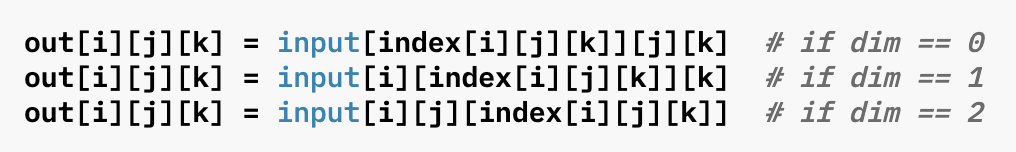
- argument 에서
t = torch.arange(24).reshape(2, 3, 4)
print(t)
# tensor([[[ 0,  1,  2,  3],
#          [ 4,  5,  6,  7],
#          [ 8,  9, 10, 11]],
#         [[12, 13, 14, 15],
#          [16, 17, 18, 19],
#          [20, 21, 22, 23]]])
print(t.dim(), t.shape)  # 3, torch.Size([2, 3, 4])

idx = torch.tensor([[[0, 1], [0, 1]], [[0, 1], [0, 1]]])
print(idx.dim(), idx.shape)  # 3, torch.Size([2, 2, 2])

print(torch.gather(t, -1, idx))
# tensor([[[ 0,  1],
#           [ 4,  5]],
#          [[12, 13],
#           [16, 17]]])
print(torch.gather(t, -1, idx).shape)  # torch.Size([2, 2, 2])
Boolean array indexing
- 비교 연산의 출력은
True/False가 나오게 되는데 이를 indexing 에 사용할 수 있다.
n = np.arange(24).reshape(2, 3, 4)
t = torch.arange(24).reshape(2, 3, 4)

print(n > 12)
# [[[False False False False]
#   [False False False False]
#   [False False False False]]
#  [[False  True  True  True]
#   [ True  True  True  True]
#   [ True  True  True  True]]]
print(t > 12)
# tensor([[[False, False, False, False],
#          [False, False, False, False],
#          [False, False, False, False]],
#         [[False,  True,  True,  True],
#          [ True,  True,  True,  True],
#          [ True,  True,  True,  True]]])
print(n[n>12])  # [13 14 15 16 17 18 19 20 21 22 23]
print(t[t>12])  # tensor([13, 14, 15, 16, 17, 18, 19, 20, 21, 22, 23])
- Integer array indexing 과 Boolean array indexing 은 Fancy indexing 이라고 불린다. 이 Fancy indexing 은 위에서 살펴본 여러 다른 indexing 과 달리 원본과 독립적인 새로운 array 혹은 tensor 를 만들어낸다.
- 이를 view 가 아닌 copy 한다고 하며, 해당 개념은 아래에서 다룰 것이다.
n = np.arange(10)
t = torch.arange(10)

n_new = n[n > 6]
t_new = t[t > 6]

n_new[0] = 100
t_new[0] = 100

print(n)      # [0 1 2 3 4 5 6 7 8 9]
print(n_new)  # [100   8   9]

print(t)      # tensor([0, 1, 2, 3, 4, 5, 6, 7, 8, 9])
print(t_new)  # tensor([100,   8,   9])
torch.item()
- 추가적으로
torch에는torch.item()이라는 함수가 있다. 이는 학습 알고리즘에 자주 사용되는 함수인데, 이를 사용하면 1개의 scalar 값으로만 이루어진 tensor 에서 값을 python number 로 가져올 수 있다.
t = torch.tensor([[[0.1223]]])
print(t.item())  # 0.12229999899864197
- 보통 학습 과정에서 loss 값을 monitoring 할 때
loss_sum += loss.item()하여 사용한다. - 그러나 이는 tensor 를 GPU 에서 CPU 로 다시 가져오는 것으로 synchronize 가 발생하여 학습에 비효율적이다.
- 실제로 pytorch 에서는 필요한 경우가 아니면 코드 상에서
.item()을 사용하지 않는 것이 좋다고 권고하고 있다. - tensor 가 GPU 상에서 CPU 로 옮기지 않은 상태에서 학습이 되지 않게 하려면
.detach()를 사용하고, numpy 로 계산이 필요하다면loss.detach().cpu().numpy()의 순서로 사용한다. - 이에 대해서는 다른 포스트를 두어 자세히 정리한다.
axis
- numpy 나 torch 는 C-order indexing 으로서, row-major 이기 때문에 맨 앞 차원부터
axis = 0이다. row-major 에 대한 것은 해당 포스트에 잘 정리했다. - numpy 와 torch 의 함수를 쓰다보면, numpy 는
axis, torch 는dim으로 사용하는 것을 볼 수 있다. 두 개념은 같은 의미다.(z, y, x)에서 z 는axis(dim) = 0이다. - 새로운 차원이 추가되면 새로운 차원의 값은 맨 앞으로 오고
axis = 0이 된다. 그리고 원래 있던 차원은 axis 가 1 씩 더해지면서 오른쪽으로 한 칸씩 이동한다. axis(dim)가 중요한 이유는 딥러닝에서torch.sum()이나torch.concat()등을 할 때 사용되는 개념이기 때문이다.
sum
sum()은 말 그대로 더하는 연산이다. 이 때axis(dim)을 어떻게 주느냐에 따라 결과가 달라진다.
p_list = [[[1,2],
           [3,4]],
           [[5,6],
           [7,8]]]
n = np.array(p_list)
t = torch.tensor(p_list)

print(n.sum())  # 36
print(n.sum(axis=0))
# [[ 6  8]
#  [10 12]]
print(n.sum(axis=1))
# [[ 4  6]
#  [12 14]]
print(n.sum(axis=-1))
# [[ 3  7]
#  [11 15]]
print(t.sum())  # tensor(36)
print(t.sum(dim=0))
# tensor([[ 6,  8],
#         [10, 12]])
print(t.sum(dim=1))
# tensor([[ 4,  6],
#         [12, 14]])
print(t.sum(dim=2))
# tensor([[ 3,  7],
#         [11, 15]])
- 위 예제를 보면 주어진
axis(dim)을 기준으로 연산이 이뤄진 것을 알 수 있다.
concatenate
- array 나 tensor 를 합치는 연산이다. 이 때
axis(dim)을 주어 어느 방향으로 합칠 것인가를 결정할 수 있다. - 딥러닝에는 모델 구조 중 단순 concatenation 하는 구조가 있다. 이 때 이 함수를 사용한다.
- numpy 에서는
np.concatenate((array1, array2), aixs)로 사용한다. - torch 에서는
torch.cat((tensor1, tensor2), dim)로 사용한다.
import numpy as np
import torch

arr1 = np.array([[1, 2], [3, 4]])
arr2 = np.array([[5, 6], [7, 8]])

# row 를 기준으로 연결 (axis=0)
concatenated_axis0 = np.concatenate((arr1, arr2), axis=0)
print(concatenated_axis0)
# [[1 2]
#  [3 4]
#  [5 6]
#  [7 8]]
print(concatenated_axis0.shape)  # (4, 2)

# column 을 기준으로 연결 (axis=1)
concatenated_axis1 = np.concatenate((arr1, arr2), axis=1)
print(concatenated_axis1)
# [[1 2 5 6]
#  [3 4 7 8]]
print(concatenated_axis1.shape)  # (2, 4)

t1 = torch.tensor([[1, 2], [3, 4]])
t2 = torch.tensor([[5, 6], [7, 8]])

# row 를 기준으로 연결 (dim=0)
concatenated_dim0 = torch.cat((t1, t2), dim=0)
print(concatenated_dim0)
# tensor([[1, 2],
#         [3, 4],
#         [5, 6],
#         [7, 8]])
print(concatenated_dim0.shape)  # torch.Size([4, 2])

# column 을 기준으로 연결 (dim=1)
concatenated_dim1 = torch.cat((t1, t2), dim=1)
print(concatenated_dim1)
# tensor([[1, 2, 5, 6],
#         [3, 4, 7, 8]])
print(concatenated_dim1.shape)  # torch.Size([2, 4])
- torch 에서는 이처럼 원하는
dim방향으로 tensor 를 쌓는 연산 뿐 아니라, 새로운 차원에 쌓는 방법도 있다. 바로stack()이다. 주의할 점은 같은 shape 의 tensor 끼리만 쌓을 수 있고dim에 기존 차원보다 두 차원 이상을 입력할 수는 없다.
t1 = torch.tensor([[1, 2, 3], [3, 4, 5]])
t2 = torch.tensor([[5, 6, 7], [7, 8, 9]])
t3 = torch.tensor([[10,11,12], [12,13,14]])

print(torch.stack((t1, t2, t3), dim=0).shape)  # torch.Size([3, 2, 3])
print(torch.stack((t1, t2, t3), dim=1).shape)  # torch.Size([2, 3, 3])
print(torch.stack((t1, t2, t3), dim=2).shape)  # torch.Size([2, 3, 3])
print(torch.stack((t1, t2, t3), dim=3).shape)
# IndexError: Dimension out of range (expected to be in range of [-3, 2], but got 3)
split
- 이는 위와 반대로 array 나 tensor 를 분리시키는 연산이다. 마찬가지로
axis(dim)을 주어 원하는 방향(차원, 축)에서 분리시킬 수 있다. - 이 함수 또한 딥러닝에서 dataset 을 나누거나 할 때 사용할 수 있다. 물론 torch 에서 메서드로 해당 기능을 지원하고 있지만, split 하는 방법을 알아두면 좋다.
- numpy 에서는
np.split(array, indices_or_sections, axis)로 사용하여 array 를 몇 개의 하위 array 로 나눌지 결정하는 index 나 개수를 건네준다. - 이 때 나누는 기준이 되는 index 를 1D array
[i, j]로 주게 되면[:i], [i:j], [j:]로 나누게 된다.
import numpy as np

arr = np.array([[1, 2, 3, 4], [5, 6, 7, 8]])

# 열을 기준으로 2개로 분할 (axis=1)
split_arr = np.split(arr, 2, axis=1)
print(split_arr)
# [array([[1, 2],
#        [5, 6]]),
#  array([[3, 4],
#        [7, 8]])]
for s in split_arr:
    print(s.shape) # (2, 2), (2, 2)

# 행을 기준으로 2개로 분할 (axis=0)
split_arr_axis0 = np.split(arr, 2, axis=0)
print(split_arr_axis0)
# [array([[1, 2, 3, 4]]), array([[5, 6, 7, 8]])]
for s in split_arr_axis0:
    print(s.shape) # (1, 4), (1, 4)

# index 로 분할
split_arr_idx = np.split(arr, [1, 2], axis=1)
print(split_arr_idx)
# [array([[1],
#        [5]]),
#  array([[2],
#        [6]]),
#  array([[3, 4],
#        [7, 8]])]
for s in split_arr_idx:
    print(s.shape) # (2, 1), (2, 1), (2, 2)

split_arr_idx_axis0 = np.split(arr, [0, 1], axis=0)
print(split_arr_idx_axis0)
# [array([], shape=(0, 4), dtype=int64), array([[1, 2, 3, 4]]), array([[5, 6, 7, 8]])]
for s in split_arr_idx_axis0:
    print(s.shape) # (0, 4), (1, 4), (1, 4)
- torch 에서는
torch.split(tensor, split_size_or_sections, dim=0)와torch.chunk(input, chunks, dim=0)가 있다. torch.split()은 주어진 차원에서 주어진 크기 만큼의 데이터가 들어있는 tensor 로 자르는 것이고,torch.chunk()는 주어진 개수가 되도록 tensor 를 자르는 것이다.- 두 함수 모두 나누다가 마지막에 데이터가 부족하면 그냥 내보낸다. 아래 예제를 보자.
import torch

t = torch.arange(24).reshape(3, 8)

split_tensor = torch.split(t, 4, dim=1)
for s in split_tensor:
    print(s.shape, end=', ') # torch.Size([3, 4]), torch.Size([3, 4])

split_tensor_dim0 = torch.split(t, 2, dim=0)
for s in split_tensor_dim0:
    print(s.shape, end= ', ') # torch.Size([2, 8]), torch.Size([1, 8])

chunk_tensor = torch.chunk(t, 3, dim=1)
for c in chunk_tensor:
    print(c.shape, end= ', ') # torch.Size([3, 3]), torch.Size([3, 3]), torch.Size([3, 2])

chunk_tensor_dim0 = torch.chunk(t, 2, dim=0)
for c in chunk_tensor_dim0:
    print(c.shape, end=', ') # torch.Size([2, 8]), torch.Size([1, 8])
copy vs. view
- numpy 와 torch 에서 자주 보이는 array 나 tensor 의 copy와 view는 array 나 tensor 의 메모리 관리를 다룰 때 중요한 개념이다. 이는 shallow copy 와 deep copy 와도 관련이 있다.
- shallow copy
- 객체를 복사할 때, 해당 객체만 복사하여 새 객체를 생성한다. 이 때 복사된 객체의 인스턴스 변수는 원본 객체의 인스턴스 변수와 같은 메모리 주소를 참조한다.
- 따라서, 해당 메모리 주소의 값이 변경되면 원본 객체 및 복사 객체의 인스턴스 변수값은 같이 변경된다.
- deep copy
- 객체를 복사 할 때, 해당 객체와 인스턴스 변수까지 같이 복사하는 방식이다.
- 이처럼 전부를 복사하여 새 주소에 담기 때문에 메모리 참조 주소를 공유하지 않는다.
- shallow copy
- numpy 와 torch 에서 copy 와 view 의 차이점은 메모리에 실제 데이터가 새로 생성되는지 여부에 있다.
numpy
- numpy 에서 view 는 array 의 데이터를 공유하는 shallow copy 를 만든다. 즉 새로운 메모리를 할당하지 않고, 기존 array 의 데이터에 대한 다른 참조(reference)만을 생성한다.
- view 는 원본 array 의 값을 변경하면 값이 같이 변경된다. 반대로, view 에서 값을 변경하면 원본 array 도 영향을 받는다.
import numpy as np

arr = np.array([1, 2, 3, 4])
view_arr = arr.view()

view_arr[0] = 100
print(arr)  # [100 2 3 4]
- copy(deep copy) 는 배열의 깊은 복사본을 생성한다. 즉 새로운 메모리를 할당하여 원본 array 의 데이터와 독립적인 새로운 array 를 만든다.
- 원본 array 와 copy 는 서로 독립적이기 때문에, 한쪽의 데이터를 변경해도 다른 쪽에 영향을 미치지 않는다.
import numpy as np

arr = np.array([1, 2, 3, 4])
copy_arr = arr.copy()

copy_arr[0] = 100
print(arr)       # [1 2 3 4]
print(copy_arr)  # [100 2 3 4]
- 위에서 살펴본 것처럼 array 에서 indexing 하거나 slicing 을 하면 view 가 생성된다. 그러나 integer indexing 이나 boolean indexing 같은 fancy indexing 은 copy 를 생성해낸다.
torch
- torch 에서 view 는 tensor 의 shape 을 변경하는데 사용되며, 이 때 원본 tensor 의 데이터를 공유하는 새로운 tensor 를 생성한다.
- numpy 의
view()와는 다르게, tensor 의 데이터 레이아웃이 연속적(contiguous)이어야만view()를 사용할 수 있다. 그렇지 않으면 오류가 발생한다. - 원본 tesnor 의 데이터를 변경하면 view tensor 의 데이터도 변경되고, 그 반대도 성립한다.
import torch

t = torch.tensor([1, 2, 3, 4])
view_t = t.view(2, 2)
view_t[0, 0] = 100
print(t)        # tensor([100,   2,   3,   4])
print(view_t)
# tensor([[100,   2],
#         [  3,   4]])
- torch 에서
clone()은 numpy 의copy()와 같은 역할을 한다. 즉 deep copy 다. - 이는 새로운 메모리에 tensor 를 복사하고, 원본 tensor 와 독립적인 tensor 를 생성한다. 이 때
detach()와 함께 사용하면 gradient 추적이 없는 복사본을 얻을 수 있다.
import torch

t = torch.tensor([1, 2, 3, 4])
clone_t = t.clone()

clone_t[0] = 100
print(t)         # tensor([1, 2, 3, 4])
print(clone_t)   # tensor([100, 2, 3, 4])

clone_t_no_graph = t.clone().detach() # clone 으로 deep copy 후 detach 로 gradient 추적 끊기
detach()는 tensor 에서 computational graph 를 분리하여 gradient 를 추적하지 않는 새로운 tensor 를 생성한다. 이 때 view 로 생성되어 데이터를 공유하기 때문에 원본 tensor 와 값이 연동된다.
t = torch.tensor([1, 2, 3, 4], requires_grad=True, dtype=torch.float32)
detach_t = t.detach()

detach_t[0] = 100
print(t)        # tensor([100.,   2.,   3.,   4.], requires_grad=True)
print(detach_t) # tensor([100.,   2.,   3.,   4.])
- numpy 와 torch 에서 copy 와 view 의 주요 차이점을 보자.
view(): 두 라이브러리 모두view()는 데이터가 공유되는 shallow copy 를 의미하지만, torch 에서는 데이터 레이아웃이 contiguous 해야 한다는 제한이 있다.copy(): numpy 에서copy()는 deep copy 를 의미하며, torch 에서 이에 대응하는 함수가clone()이다.detach(): GPU 사용에 특화되어 있는 torch 에서만 있는 함수로,detach()는 gradient 를 추적하지 않는 새로운 tensor 를 shallow copy 로 생성한다.
Tensor rank/shape 조작
- 여기서는 torch 의
torch.Tensor가 가진 rank / shape 을 조작하는 법을 다뤄보자. 여기서는view(),reshape(),transpose(),permute(),squeeze(),unsqueeze(),flatten()을 다룰 것이다. - 또한 위에서 view 와 copy 를 다룰 때 살짝 언급했던 numpy 와 torch 의 contiguous 성질에 대해 알아보자.
view vs. reshape
torch.view()와torch.reshape()는 torch 에서 tensor 의 모양(shape)을 변경하는 두 가지 주요 메서드다.- 두 메서드 모두 원본 tensor 를 새로운 모양의 tensor 로 반환하지만, 내부적으로 약간 다르게 작동하고 특정 상황에서만 교환하여 사용할 수 있다.
- 먼저
torch.view()는 tensor 의 메모리에서 연속된 데이터를 기반으로 새로운 모양을 반환한다. 즉, 원래 tensor 가 contiguous(연속된 메모리 배열)일 때만 새로운 tensor 를 생성할 수 있다. - 만약 tensor 가 contiguous 하지 않다면, 먼저
.contiguous()메서드를 사용해 연속적인 tensor 로 만든 후view()를 사용해야 한다. - 이처럼
view()는 원본 데이터의 메모리 배치를 변경하지 않고, tensor 의 모양만 바꾸는 방식으로 작동하므로 새로운 메모리를 할당하는 것 없이 효율적이다. - 쉽게 말해, 원본 데이터의 메모리 배치에서 읽는 순서를 바꾸어 마치 tensor 의 shape 과 차원이 변경된 것처럼 만드는 것이다. 따라서
view()는 원본 데이터와 독립적이지 않은 shallow copy 에 해당한다.
import torch

tensor = torch.tensor([[1, 2, 3], [4, 5, 6]])
print(tensor.shape)  # torch.Size([2, 3])

viewed_tensor = tensor.view(1, 6)
print(viewed_tensor)  # tensor([[1, 2, 3, 4, 5, 6]])

tensor[0][0] = 100
viewed_tensor[-1][-1] = 100
print(tensor)
# tensor([[100,   2,   3],
#         [  4,   5, 100]])
print(viewed_tensor)
# tensor([[100,   2,   3,   4,   5, 100]])
- 반면에
torch.reshape()는view()와 유사하게 tensor 의 모양을 변경하지만, contiguous 여부에 상관없이 사용할 수 있다. - 따라서
reshape()는 메모리에서 연속되지 않은(non-contiguous) tensor 라도 새로운 모양으로 쉽게 변환할 수 있다. - 주의할 점은, contiguous 한 tensor 의 경우
view()와 같이 shallow view 가 된다. - 반대로 contiguous 한 tensor 가 아닌 경우, 내부적으로
reshape()는 deep copy 가 되어 원래 tensor 를 복사하여 새로운 연속적인 메모리 배열로 만든 후 변환을 수행한다. - 이처럼 연속적이지 않은 메모리 구조를 가진 tensor 가 있을 때
reshape()를 사용하여 해당 tensor 의 shape 을 변경할 수 있어view()보다 유연하지만, 추가적인 메모리 비용이 발생할 수 있다. - 아래 예제를 보자.
.data_ptr()은 tensor 의 데이터가 저장된 메모리의 시작 주소를 반환하기 때문에, 두 tensor 의.data_ptr()값이 같다면 같은 메모리를 공유하고 있다는 것을 의미한다. - 또한
.is_contiguous()는 해당 tensor 가 메모리에서 contiguous 한 tensor 인지를True / False로 반환한다.
import torch

tensor = torch.tensor([[1, 2, 3], [4, 5, 6]])
tensor_t = torch.transpose(tensor, 0, 1)  # 전치연산
print(tensor.shape, tensor.is_contiguous())      # torch.Size([2, 3]) True
print(tensor_t.shape, tensor_t.is_contiguous())  # torch.Size([3, 2]) False

reshaped_tensor = tensor.reshape(1, 6)
reshaped_tensor_t = tensor_t.reshape(1, 6)
print(reshaped_tensor, reshaped_tensor.is_contiguous())
# tensor([[1, 2, 3, 4, 5, 6]]) True
print(reshaped_tensor_t, reshaped_tensor_t.is_contiguous())
# tensor([[1, 4, 2, 5, 3, 6]]) True

tensor[0][0] = 100

print(tensor)
# tensor([[100,   2,   3],
#         [  4,   5,   6]])
print(tensor_t)
# tensor([[100,   4],
#         [  2,   5],
#         [  3,   6]])
print(reshaped_tensor)   # tensor([[100,   2,   3,   4,   5,   6]])
print(reshaped_tensor_t) # tensor([[1, 4, 2, 5, 3, 6]])

print(tensor.data_ptr() == tensor_t.data_ptr())             # True
print(tensor.data_ptr() == reshaped_tensor.data_ptr())      # True
print(tensor.data_ptr() == reshaped_tensor_t.data_ptr())    # False
print(tensor_t.data_ptr() == reshaped_tensor_t.data_ptr())  # False
- 정리하면, contiguous 한 tensor 를 빠르게 변형하고 싶다면
view()가 더 효율적이다. 왜냐하면 메모리 할당이 필요하지 않기 때문이다. - 반대로 non-contiguous tensor 이거나, 차원 변환을 적용하려는 tensor 의 상태에 대하여 정확하게 파악하기가 모호한 경우
reshape()가 적합하다. - 추가적으로 이러한 shape 변경에는 1 개의 dim 에 한해서
-1을 사용할 수 있다. 이는 shape 을 변형하더라도 총 dim 의 수는 동일하기 때문에-1을 건네받은 dim 은 남은 차원 수를 유추하여 자동으로 채워진다.
import torch

tensor = torch.arange(24).view(2, 3, 4)
viewed_tensor = tensor.view(4, 6, -1)
reshaped_tensor = tensor.reshape(3, -1, 2)

print(viewed_tensor.shape)   # torch.Size([4, 6, 1])
print(reshaped_tensor.shape) # torch.Size([3, 4, 2])
transpose vs. permute
transpose()와permute()는 tensor 의 차원 순서를 변경할 때 자주 사용하는 메서드다. 이 때 사용 방식과 유연성에서 약간의 차이가 있다.- 두 메서드 모두 tensor 의 데이터 내용과 메모리 참조는 유지하면서 차원의 순서만 바꾼다. 즉 view 를 생성하는 것과 같다. 또한 두 메서드는 모두 tensor 의 contiguous 와 상관없이 사용할 수 있다.
- 그러나 반환값 결과에 따라 non-contiguous 할 수도 contiguous 할 수도 있다. 즉 반환된 결과가 원본 tensor 와 같아지면 contiguous 해질 수 있다.
transpose(dim0, dim1)는 두 개의 차원을 교환(swap)한다. 즉, tensor 의 두 축을 선택해서 그 두 축의 위치만 서로 바꿀 수 있다.- 여러 차원을 동시에 변경할 수 없고, 두 차원만 교환이 가능하므로 여러 차원을 동시에 바꾸려면 여러 번
transpose()를 호출해야 한다. - 반면에
permute(dims)는 tensor 의 모든 차원을 임의 순서로 재배치할 수 있다. argument 의dims에서 주어진 순서에 따라 다차원 tensor 의 축을 원하는 대로 지정할 수 있기 때문에,transpose()보다 유연성이 높다. - 따라서
permute()는 여러 차원이 있는 고차원 tensor 에서 여러 축을 복잡하게 재배치하는 데 주로 사용된다.
import torch

tensor = torch.randn(2, 3, 4)
print(tensor.is_contiguous())  # True

transposed_tensor = tensor.transpose(0, 1)
print(transposed_tensor.shape)  # torch.Size([3, 2, 4])
print(transposed_tensor.is_contiguous()) # False

permuted_tensor = tensor.permute(1, 0, 2)
print(permuted_tensor.shape)  # torch.Size([3, 2, 4])
print(permuted_tensor.is_contiguous()) # False

permuted_tensor2 = transposed_tensor.permute(1, 0, 2)
print(permuted_tensor2.shape) # torch.Size([2, 3, 4])
print(permuted_tensor2.is_contiguous()) # True
- 정리하면, 이 두 함수는 데이터의 구조를 재배치하여 tensor 의 shape 을 변환시켜주며, 원본 tensor 와 메모리를 공유하는 view 를 반환한다.
- 행렬의 전치(행과 열을 교환) 및 두 축만 변경이 필요한 경우
transpose()를 사용하고, 다차원 tensor 에서 다양한 차원의 순서를 필요로 할 때(image 데이터를 C-H-W 에서 H-W-C 순으로 변경)permute()를 사용한다.
contiguous
- contiguous 에 대한 설명은 해당 포스트에서 잘 정리했지만 여기서 다시 한 번 살펴보자.
-
기본적으로
torch.Tensor는 생성될 때부터 row-major 로 contiguous 하다. 즉 row 방향으로 메모리 주소가 연속적이다.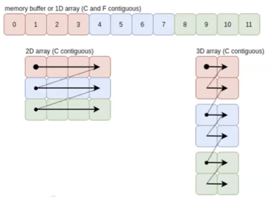
- 이는 메모리 효율성과 직결된다. 원본 tensor 와 메모리는 공유하는데 contiguous 를 non-contiguous 로 바꾼 view 를 사용함으로써 매번 새로운 메모리에 할당해야 하는 소요를 줄일 수 있다.
- 즉 차원의 순서를 뒤집거나 읽는 방향을 뒤집거나 하는 연산 처리를 했을 때 불연속(non-contiguous)적인 view 를 만들고, 기저에 있는 메모리는 동일하게 있는데 메모리를 읽는 방식을 바꿈으로써 2차원 tensor 를 3차원 tensor 로 바꾼다던지, Transpose 연산을 적용한다던지 할 수 있다.
- 우리는 위에서
transpose()나permute()의 반환값이 non-contiguous 함을 봤다. 아래 예제를 보자. - tensor 가 contiguous 한지는
is_contiguous()를 통해 알 수 있다.
import torch

tensor = torch.arange(6, dtype=torch.float32).view(2, -1)
print(tensor.is_contiguous())   # True
for i in range(tensor.shape[0]):
    for j in range(tensor.shape[1]):
        print(tensor[i][j].data_ptr())
# 4365408576
# 4365408580
# 4365408584
# 4365408588
# 4365408592
# 4365408596

tensor_transpose = tensor.transpose(1, 0)
print(tensor_transpose.is_contiguous())   # False
for i in range(tensor_transpose.shape[0]):
    for j in range(tensor_transpose.shape[1]):
        print(tensor_transpose[i][j].data_ptr())
# 4365408576
# 4365408588
# 4365408580
# 4365408592
# 4365408584
# 4365408596
- 위 예제를 보면 자료형을
dtype = torch.float32로 하여 데이터 하나 당 32 bit 다. 따라서 메모리 한 칸에는 8 bit 당 1 byte 이므로 4 byte 씩 가지고 있다. torch.arange()로 생성한 tensor 는 contiguous 하여 데이터를 row-major 로 읽었을 때 4 byte 씩 균일하게 증가한다.- 그러나
transpose()를 취한 결과로 non-contiguous 한 view 를 얻었으므로, 메모리 주소 값은 동일하지만 순서가 다르게 되어 있음을 볼 수 있다. 이를 통해 동일한 메모리를 가지고 있지만 메모리를 읽는 방식을 바꾼 것을 알 수 있다. - 이를 알 수 있는 또 다른 방법은
stride()를 이용하는 것이다.
print(tensor.stride())           # (3, 1)
print(tensor_transpose.stride()) # (1, 3)
- 위 결과에서
(3, 1)은tensor[0][0]에서tensor[1][0]으로 갈 때는 데이터 3 개 만큼의 메모리 주소가 이동하고,tensor[0][0]에서tensor[0][1]으로 갈 때는 데이터 1 개 만큼의 메모리 주소가 이동한다는 뜻이다. - 즉 메모리 주소를 순서대로 옮겨가며 3 번 읽을 때마다 다음 데이터 포인트로 넘어간다는 것이다. 이를 통해 tensor 가 어느 방향으로 읽히는지 알 수 있다.
- 추가적으로 non-contiguous 한 tensor 에
contiguous()메서드를 이용하면 contiguous 하게 바꿀 수 있다.
import torch

tensor = torch.randn(3, 5)
transposed_tensor = tensor.transpose(0, 1)
print(transposed_tensor.is_contiguous()) # False

transposed_tensor = transposed_tensor.contiguous()
print(transposed_tensor.is_contiguous()) # True
squeeze, unsqueeze, flatten
torch.squeeze,torch.unsqueeze,torch.flatten또한 모두 tensor 의 차원을 변경하는데 사용되는 함수로 딥러닝에서 많이 사용된다.torch.squeeze(tensor, dim)는 tensor 에서 크기가 1인 차원을 제거한다. 이 때, 특정 차원만 제거하고 싶다면dimparameter 를 사용할 수 있다.- 예를 들어,
torch.squeeze(tensor, dim=0)은 0 번째 차원이 1 일 때만 제거한다. - 반대로
torch.unsqueeze(tensor, dim)는 tensor 에 크기가 1 인 차원을 추가한다. 추가된 차원은 특정 dim 위치에 삽입된다. - 예를 들어,
torch.unsqueeze(tensor, dim=1)이라면(3, 5)가(3, 1, 5)가 된다. 이는 차원을 늘려서 batch 처리를 하거나 브로드캐스팅을 할 때 유용하다. 단, 차원의 수를 1 개만 늘릴 수 있다. torch.flatten(input, start_dim=0, end_dim=-1)은 tensor 를 1차원 vector 로 평탄화한다. Fully Connected Layer 에서 자주 사용된다.- 특정 차원만 평탄화하고 싶다면
start_dim과end_dimparameter 로 범위를 지정할 수 있다. 예를 들어,torch.flatten(tensor, start_dim=1)은(2, 3, 4)를(2, 12)로 만든다.
import torch

## squeeze
tensor = torch.rand(1, 3, 1, 5)
squeezed_tensor = torch.squeeze(tensor)
print(squeezed_tensor.shape) # torch.Size([3, 5])

## unsqueeze
tensor = torch.rand(3, 5)
unsqueezed_tensor1 = torch.unsqueeze(tensor, dim=0)
unsqueezed_tensor2 = torch.unsqueeze(tensor, dim=2)
print(unsqueezed_tensor1.shape) # torch.Size([1, 3, 5])
print(unsqueezed_tensor2.shape) # torch.Size([3, 5, 1])

## flattem
tensor = torch.rand(2, 3, 4)
flattened_tensor1 = torch.flatten(tensor)
flattened_tensor2 = torch.flatten(tensor, start_dim=0, end_dim=1)
print(flattened_tensor1.shape) # torch.Size([24])
print(flattened_tensor2.shape) # torch.Size([6, 4])
댓글 남기기