
[Pytorch] Pytorch 기본 및 Tensor 연산
이 포스트에서는 Pytorch 가 무엇인지 좀 더 자세히 알아보고, 딥러닝의 근간이 되는 다양한 행렬 연산을 어떤 함수로 정의했는지 정리할 것이다. 또한 추가적으로 Pytorch 를 사용할 때 사용하는 세팅을 살펴보자.
Pytorch 기본
- 먼저 Pytorch 에 대해 알아보자. Pytorch 는 2016년 Facebook AI Research(FAIR) 에서 Torch7 이라는 Lua 기반 딥러닝 프레임워크로 만들어졌다. 이후 효율성과 배포 가능성에 중점을 둔 Caffe2 와 통합되면서 현재의 Pytorch 가 되었다.
- Pytorch 는 이름처럼 Python 을 기반으로 사용하며, 진화된 Torch C/CUDA 백엔드를 사용한다.
- 흔히 Pytorch 를 “강력한 GPU 가속이 적용되는 Python 으로 된 Tensor 와 동적 신경망”이라고 하는데, 이것이 무슨 뜻일까?
- Tensor 는 물리학과 공학에 많이 사용되는 수학적 구조다. Rank 2 의 Tensor 는 특수한 종류의 Matrix 로, Vector 의 내적(inner product)을 취하면서 새로운 크기와 새로운 방향으로 다른 Vector 를 산출한다.
- 참고로 Tensorflow 는 Tensor 가 네트워크 모델을 따라 흐른다는 데서 이름을 따왔다. Numpy 역시 Tensor 를 사용하지만
ndarray라는 명칭을 사용한다. - GPU 가속(GPU acceleration)은 대부분의 현대 딥러닝 프레임워크가 가지고 있는 기능이다. 이 때 Pytorch 의 동적 신경망(dynamic neural network)은 반복할 때마다 변경이 가능한 신경망으로, 예를 들어 Pytorch 모델이 학습 중 hidden layer 을 추가하거나 제거해서 정확성과 일반성을 개선할 수 있도록 한다.
- 이는 Pytorch 가 각 epoch 단계에서 즉석으로 Computational Graph 를 재생성한다는 의미다. 반면 Tensorflow 는 기본적으로 단일 데이터 흐름 그래프를 만들고 그래프 코드를 성능에 맞게 최적화한 다음 모델을 학습시킨다는 점에서 차이가 있다.
- 또한 Pytorch 의 경우, Tensorflow 와 달리 즉시 실행(Eager Execution)이 유일한 실행 방법이다. API 호출은 그래프에 추가되어 나중에 실행되는 것이 아니라 호출 시 바로 실행된다.
- 얼핏 계산 측면에서 효율성이 낮을 것 같지만 Pytorch 는 원래 그런 방식으로 동작하도록 설계됐으며, 학습 및 예측 속도 측면에서 봐도 느리지 않다.
- 추가로 Pytorch 는 속도를 극대화하기 위해 intel MKL, Nvidia CuDNN, NCCL 과 같은 가속 라이브러리를 통합했다. 코어 CPU 와 GPU Tensor 및 신경망 백엔드들은 C99 API 를 사용해 독립적인 라이브러리로 작성된다.
- 이처럼 Pytorch 는 모놀리식 C++ 프레임워크에 대한 Python 바인딩이 아니다. Python 과 심층적으로 통합되고 다른 Python 라이브러리를 사용할 수 있도록 하기 위해서다.
Pytorch 구성요소
torch- main namespace 인 torch 패키지는 다차원 tensor 를 위한 데이터 구조를 포함하고, 이러한 tensor 에 대한 수학적 연산을 정의한다.
- tensor 와 numpy 와 같은 임의의 타입을 효율적으로 serialization 할 수 있는 여러 유틸리티와 유용한 도구를 제공한다.
- 특히 numpy 와 비슷한 구조를 가지고 있어서 문법 구조 또한 비슷하다.
torchvision- 많이 사용되는 데이터셋, Classification, Detection, Segmentation 과 같은 다양한 task 의 pre-trained 모델 아키텍처를 제공하고, 이미지 변환(transform) 기능들로 구성되어 있다.
torch.nn- 그래프의 구성 요소가 Module 로 정의되어 있다. 즉 신경망을 구축하기 위한 다양한 데이터 구조나 layer 가 정의되어 있다. 따라서 모델링을 할 때 가장 많이 사용하게 된다.
- Convolution(
Conv2d), Recurrent(LSTM), 활성화 함수(ReLu), loss(BCELoss) 등이 정의되어 있다.
torch.autograd- 자동 미분을 위한 함수가 포함되어 있으며, 임의의 스칼라 값을 내는 함수를 자동으로 미분하는 클래스를 제공한다.
- 기존 코드에 최소한의 변경만 필요하다. 즉 tensor 에
requires_grad=Trueargument 를 사용하여 미분값을 계산할 tensor 를 선언하면 된다. - 현재로서는 부동소수점 tesnor 타입(half, float, double, bfloat16)과 복소수 tensor 타입(cfloat, cdouble)에 대해서만 자동 미분을 지원한다.
- 자동 미분의 on, off 를 제어하는
enable_grad또는no_grad나 자체 미분 가능 함수를 정의할 때 사용하는 기반 클래스인 Function 등이 포함된다.
torch.optim- 다양한 최적화 알고리즘을 구현하는 패키지다. SGD 등의 parameter 최적화(optimization) 알고리즘들이 구현되어 있다.
- 즉 많이 사용되고 있는 최적화 방법들을 지원하며, 인터페이스가 일반화되어 있어 더욱 정교한 방법들도 쉽게 통합할 수 있다.
torch.utils.data- PyTorch 의 데이터 로딩 유틸리티의 중심에는
torch.utils.data.DataLoader클래스가 있다. 이 클래스는 데이터셋에 대한 Python iterable 을 나타낸다. - 즉 반복 연산을 할 때 사용하는 mini-batch 용 유틸리티 함수가 포함되어 있다.
__getitem__(), __len__()를 가지고 데이터 샘플에 대해 index 로 접근할 수 있는 map-style 및__iter__()를 통해 데이터 샘플을 반복적으로 불러올 수 있는 iterable-style 데이터셋을 지원한다.- 또한 데이터 로딩 순서를 사용자가 지정할 수 있고, 자동 batch 처리, 단일 및 다중 프로세스 데이터 로딩, 자동 메모리 고정(pin-memory) 등을 지원한다.
- 이러한 옵션은 DataLoader 를 생성할 때 argument 를 통해 구성된다.
- PyTorch 의 데이터 로딩 유틸리티의 중심에는
torch.amp- mixed precision 을 위한 편의 메서드를 제공한다.
- mixed precision 은 일부 연산에
torch.float32(float) data type 을 사용하고, 다른 연산에 낮은 정밀도의 부동소수점 data type (lower_precision_fp), 예를 들어torch.float16(half) 또는torch.bfloat16을 사용하는 것이다. - linear layer 와 convolution 같은 연산은 낮은 정밀도에서 훨씬 빠르다. 반면에, reduction 과 같은 합산 연산은 종종 float32 의 범위를 요구한다.
- mixed precision 은 각 연산에 적합한 data type 을 맞추는 것을 목표로 한다. 보통 auto mixed precision training(amp) 은
torch.float16data type 을 사용하며,torch.autocast와torch.amp.GradScaler를 함께 사용하는 방식으로 이루어진다. - 또한
torch.autocast와torch.GradScaler는 모듈식으로 설계되어 있어 별도로 사용할 수도 있다. torch.bfloat16data type 을 사용하는 CPU 에서의 auto mixed precision training/inference 는torch.autocast만 사용한다.
torch.onnx- ONNX(Open Neural Network eXchange) 는 머신러닝 모델을 표현하기 위한 표준 형식이다. 즉, ONNX 는 서로 다른 딥러닝 프레임워크 간에 모델을 공유할 때 사용하는 새로운 포맷이다.
torch.onnx모듈은 PyTorch 의torch.nn.Module모델에서 계산 그래프를 캡처하여 ONNX 그래프로 변환한다.- 내보낸 모델은 Microsoft 의 ONNX Runtime 을 포함한 ONNX 를 지원하는 다양한 런타임에서 사용할 수 있다.
- ONNX export API 에는 두 가지 유형이 있으며, 두 가지 모두
torch.onnx.export()함수를 통해 호출할 수 있다.
Tensor 생성과 Data Type
- 먼저,
torch.Tensor와numpy.ndarray는 자유롭게 호환되지만, GPU 에 올라가있는 tensor 를numpy.ndarray로 변환하려면 CPU 로 이동한 후에 변환할 수 있다.
# tensor 를 ndarray 로 변환
t = torch.tensor([[1,2],[3,4.]])
x = t.numpy()

# GPU 상의 tensor 는 to() 혹은 cpu() 로 CPU 상 tensor 로 옮긴 후 ndarray 로 변환해야 한다.
t = torch.tensor([[1,2],[3,4.]], device="cuda:0")
x = t.to("cpu").numpy()
x = t.cpu().numpy()

# GPU 위에서 tensor 생성
t = torch.tensor([[1,2],[3,4.]], device="cuda:0")
- 여기서 GPU 와 CPU 사이의 data transfer 는 GPU 와 CPU 의 async 를 방해하고 synchronize 시키기 때문에 코드 상에서 이러한 작업을 피해야 한다.
- 또한 GPU tensor 를 사용해야 한다면 tensor 를 생성할 때 GPU 위에서 생성하는 것이 좋다.
- 이에 대한 것은 이 포스트에 잘 정리해뒀다.
np.linspace(start, stop, num)와 같이torch.linspace(start, end, steps)도 시작과 끝을 포함하고 step 의 수만큼 원소를 가진 등차수열을 만들어낸다.
print(np.linspace(0,10,2)) # [0. 10.]
print(torch.linspace(0,10,2)) # tensor([ 0., 10.])
- 또한
.randperm(n)을n보다 작은 수를 이용하여 랜덤 순열을 생성해낼 수도 있다.
torch.randperm(10)
# tensor([5, 7, 4, 8, 6, 0, 3, 9, 1, 2])
-
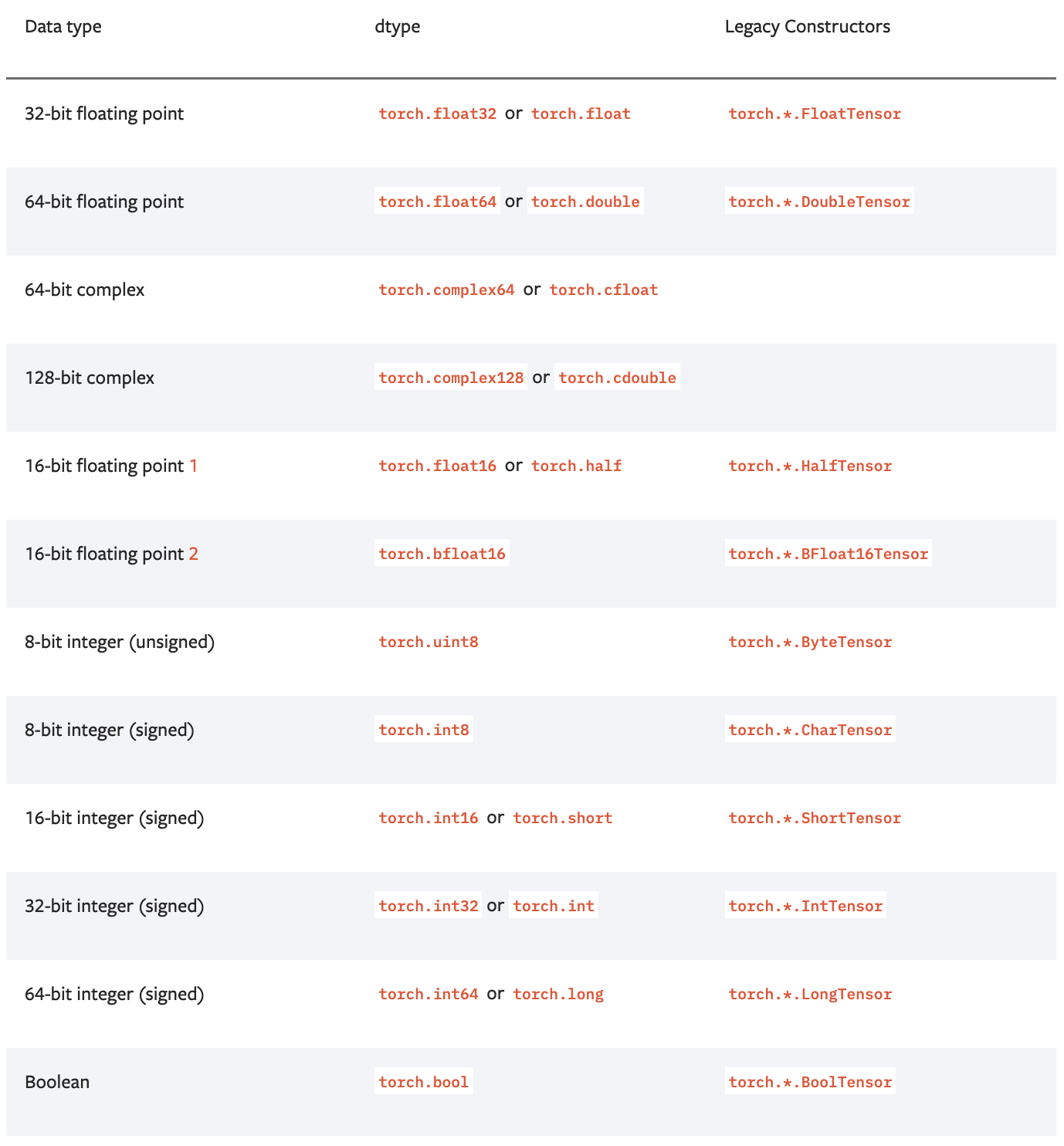
Pytorch 에서는 아래와 같은 data type 을 지원한다.
-
이러한 data type 은 tensor 를 생성할 때
dtype=으로 지정해주거나,to(dtype)혹은type(),type_as(other)를 통해 변경할 수 있다.
t_int = torch.tensor([1,2], dtype=torch.int32)
t_float = t_int.to(torch.float64)
t_half = t_int.type_as(torch.tensor([1, 2], dtype=torch.half))
t_double = t_int.type(torch.double)

print(t_int.dtype, t_float.dtype, t_half.dtype, t_double.dtype)
# torch.int32 torch.float64 torch.float16 torch.float64
- 산술 연산(
add, sub, div, mul)의 입력 data type 이 서로 다른 경우, 아래의 규칙에 따라 최소한의 data type 으로 승격(promote)이 이루어진다.- data type 의 카테고리는 순서를 가진다. 복소수(complex) > 부동소수점(float) > 정수(integral) > 불리언(boolean) 순이다. 그리고 bit 의 수도 큰 수가 더 높은 카테고리에 속하게 된다.
- data type 승격은 연산의 결과를 정확하게 유지하기 위해 높은 카테고리의 타입으로 변환하는 방식으로 동작한다.
- 스칼라의 data type 이 tensor 의 data type 보다 더 높은 카테고리에 속하는 경우, 해당 카테고리의 모든 스칼라를 담을 수 있는 충분한 크기의 data type 으로 승격한다.
- 0 차원 tensor 가 차원을 가진 tensor 보다 더 높은 카테고리에 속하는 경우, 해당 카테고리의 모든 0 차원 tensor 를 담을 수 있는 충분한 크기와 카테고리의 data type 으로 승격한다.
- 더 높은 카테고리의 0 차원 연산자가 없을 경우, 차원을 가진 모든 tensor 를 담을 수 있는 충분한 크기와 카테고리의 data type 으로 승격한다.
- 부동소수점 스칼라 연산자의 data type 은
torch.get_default_dtype()즉torch.float32이며, 정수형(non-boolean) 스칼라 연산자의 data type 은torch.int64이다. - 또한 Pytorch 는 Numpy 와는 달리, 연산자의 최소 data type 을 결정할 때 값을 검사하지 않는다. Quantized data type 과 Complex 타입은 아직 지원되지 않는다.
float_tensor = torch.ones(1, dtype=torch.float)
double_tensor = torch.ones(1, dtype=torch.double)
complex_float_tensor = torch.ones(1, dtype=torch.complex64)
complex_double_tensor = torch.ones(1, dtype=torch.complex128)
int_tensor = torch.ones(1, dtype=torch.int)
long_tensor = torch.ones(1, dtype=torch.long)
uint_tensor = torch.ones(1, dtype=torch.uint8)
double_tensor = torch.ones(1, dtype=torch.double)
bool_tensor = torch.ones(1, dtype=torch.bool)
long_zerodim = torch.tensor(1, dtype=torch.long)
int_zerodim = torch.tensor(1, dtype=torch.int)

torch.add(5, 5).dtype  # torch.int64
# 스칼라 5 는 int64 지만, int_tensor(int32) 보다 높은 카테고리가 아니라 고려되지 않는다. 만약 스칼라가 아닌 int64 의 tensor 라면 int64 가 된다.
(int_tensor + 5).dtype # torch.int32
(int_tensor + long_zerodim).dtype # torch.int32
(long_tensor + int_tensor).dtype # torch.int64
(bool_tensor + long_tensor).dtype # torch.int64
(bool_tensor + uint_tensor).dtype # torch.uint8
(float_tensor + double_tensor).dtype # torch.float64
(complex_float_tensor + complex_double_tensor).dtype # torch.complex128
(bool_tensor + int_tensor).dtype # torch.int32
torch.add(long_tensor, float_tensor).dtype # torch.float32 -> long(int64) 은 float 와 다른 카테고리이기 때문에 더 높은 카테고리인 float 를 담을 수 있는 데이터 타입이 된다.
- 만약 산술 연산의 출력 tensor data type 이 지정된 경우, 해당 데이터 타입으로 캐스팅을 허용한다. 다만, 아래의 예외 사항이 있다.
- 정수형 출력 텐서는 부동소수점 텐서를 받을 수 없다.
- boolean 형 출력 텐서는 non-boolean 텐서를 받을 수 없다.
- non-complex 형 출력 텐서는 complex 텐서를 받을 수 없다.
# allowed
float_tensor *= float_tensor
float_tensor *= int_tensor
float_tensor *= uint_tensor
float_tensor *= bool_tensor
float_tensor *= double_tensor
int_tensor *= long_tensor
int_tensor *= uint_tensor
uint_tensor *= int_tensor

# disallowed -> RuntimeError: result type can't be cast to the desired output type
int_tensor *= float_tensor
bool_tensor *= int_tensor
bool_tensor *= uint_tensor
float_tensor *= complex_float_tensor
- 마지막으로 생성자를 통해 CPU 와 GPU 에 tensor 를 생성했을 때를 보자.
x = torch.FloatTensor([[1,2,3],[4,5,6]])
x_gpu = x.to('mps') # m1 macbook mps 로 대체
print(x_gpu, x_gpu.dtype, x_gpu.type())
# tensor([[1., 2., 3.],
#         [4., 5., 6.]], device='mps:0') torch.float32 torch.mps.FloatTensor
x_cpu = x_gpu.cpu()
print(x_cpu, x_cpu.dtype, x_cpu.type())
# tensor([[1., 2., 3.],
#         [4., 5., 6.]]) torch.float32 torch.FloatTensor
- 그러나 위에서 언급한 것처럼 생성 시에
device=를 GPU 로 주어 GPU 위에 direct 하게 생성하는 것이 좋다. - 추가적으로
torch.Tensor와torch.tensor의 차이는 아래와 같다.torch.Tensor- 클래스 (Class)
- int 입력 시 float 으로 변환
- torch 데이터 입력 시 입력 받은 데이터의 메모리 공간을 사용
- list, numpy 데이터 입력 시 입력 받은 데이터를 복사하여 새롭게
torch.Tensor를 만든 후 사용
torch.tensor- 함수 (Function)
- int 입력시 int 그대로 입력
- 입력 받은 데이터를 새로운 메모리 공간으로 복사 후 사용
# torch.Tensor
original_data = torch.Tensor([1])
new_data = torch.Tensor(original_data) # torch.Tensor 를 입력 받음
print(f"original : {original_data} new : {new_data}")
# original : tensor([1.]) new : tensor([1.])
original_data[0] = 2
print(f"original : {original_data} new : {new_data}")
# original : tensor([2.]) new : tensor([2.])

original_data = [1]
new_data = torch.Tensor(original_data) # list, numpy 를 입력 받음
print(f"original : {original_data} new : {new_data}")
# original : [1] new : tensor([1.])
original_data[0] = 2
print(f"original : {original_data} new : {new_data}")
# original : [1] new : tensor([1.])

# torch.tensor - [torch.Tensor 입력]
original_data = torch.tensor([1])
new_data = torch.tensor(original_data)
print(f"original : {original_data} new : {new_data}")
# original : tensor([1]) new : tensor([1])
original_data[0] = 2
print(f"original : {original_data} new : {new_data}")
# original : tensor([2]) new : tensor([1])
tensor 의 index / shape(rank) 조작
- tensor 의 index 를 조작하는 방법은 여러가지가 있다. 이전 포스트에서 정리했지만, 여기서 간단하게 코드로 정리해보고 가자.
- tensor 는
numpy.ndarray와 index 조작법이 거의 같다. 배열처럼 index 를 바로 지정할 수도 있고, slice, mask 배열을 사용할 수 있다.
t = torch.tensor([[1,2,3],[4,5,6.]])

# index 접근
t[0, 2] # tensor(3.)

# slice 로 접근
t[:, :2] # tensor([[1., 2.], [4., 5.]])

# mask 배열을 이용하여 True 값만 추출
t[t > 3] # tensor([4., 5., 6.])

# slice 를 이용하여 일괄 대입
t[:, 1] = 10

# mask 배열을 사용하여 일괄 대입
t[t > 5] = 20
- tensor 의 차원을 변경하는
view나 tensor 를 결합하는stack,cat, 차원을 교환하는t,transpose또한 이미 전 포스트에 정리봤다.view는 numpy 의reshape과 유사하다. Pytorch 에도reshape메서드가 존재하는데 이에 대한 비교는 이후 포스트에서 자세히 정리할 예정이다.- 결국 contiguous 여부에 영향받지 않는
reshape를 사용하길 권장하지만, 만약 contiguous 한 tensor 임을 명확히 알고 있다면 추가적인 메모리 비용이 발생하지 않는view가 더 좋다. - 이 때
-1을 사용하면 shape 에서 자동 계산 가능한 부분에 한해서 자동으로 입력된다. 계산이 불가능하면 오류가 발생한다. cat은 다른 길이의 tensor 를 하나로 묶을 때 사용한다.transpose는 행렬의 전치 외에도 두 차원의 순서만을 변경할 때에도 사용된다.
x1 = torch.tensor([[1, 2], [3, 4.]])
x2 = torch.tensor([[10, 20, 30], [40, 50, 60.]])

x1.view(4,1)
# tensor([[1.],
#         [2.],
#         [3.],
#         [4.]])
x1.reshape(4,1)
# tensor([[1.],
#         [2.],
#         [3.],
#         [4.]])
x1.view(-1) # tensor([1,2,3,4])
x1.reshape(-1) # tensor([1,2,3,4])
x1.view(1, -1)
# tensor([[1.],
#         [2.],
#         [3.],
#         [4.]])
x1.reshape(1, -1)
# tensor([[1.],
#         [2.],
#         [3.],
#         [4.]])
x2.t()
# tensor([[10., 40.],
#         [20., 50.],
#         [30., 60.]])
torch.cat([x1, x2], dim=1) # stack 은 shape 이 같은 tensor 끼리만 쌓을 수 있다.
# tensor([[ 1.,  2., 10., 20., 30.],
#         [ 3.,  4., 40., 50., 60.]])
hwc_img_data = torch.rand(100, 64, 32, 3)
chw_img_data = hwc_img_data.transpose(1,2).transpose(1,3)
chw_img_data.size()
# torch.Size([100, 3, 64, 32])
- 추가적으로
torch.transpose(input, dim0, dim1)는 교환하고 싶은 2 개의 dimension 을 1:1 교환하는 방법이었다면,.permute(input, dims)를 이용하면 차원의 순서를 한번에 쉽게 바꿀 수 있다.
A = torch.ones(1, 3, 10, 20)
print(A.shape) # torch.Size([1, 3, 10, 20])

A = A.permute(1, 3, 0, 2)
print(A.shape) # torch.Size([3, 20, 1, 10])
- 위 예시와 같이 tensor 에
.permute(dims)메서드를 사용하면 기존 dimension 의 index 를 순서를 바꾼 위치에 그대로 적으면 된다. - 만약 위 예제에서
A.permute(0, 1, 2, 3)로 입력하면 차원 순서의 변경은 없고A.permute(3, 2, 1, 0)로 입력하면 차원이 완전히 반대로 변경된다. torch.t()를 이용해서도 transposed tensor 를 구할 수 있다. 반면torch.transpose()를 이용하면 특정 dimension 을 transpose 할 수 있다.
x1 = torch.FloatTensor(2,3)
x2 = x1.t()
print(x1.size()) # torch.Size([2, 3])
print(x2.size()) # torch.Size([3, 2])

x1 = torch.FloatTensor(10,3,4,5)
x1.size() # torch.Size([10, 3, 4, 5])
torch.transpose(x1,1,2).size() # torch.Size([10, 4, 3, 5])
torch.transpose(x1,2,3).size() # torch.Size([10, 3, 5, 4])
torch.index_select(input, dim, index)와torch.masked_select(input, mask)로도 indexing 및 slicing 을 할 수 있다.- 이 때
torch.index_select의index는 1D tensor 여야 한다.
x = torch.rand(4,3)
# tensor([[0.6615, 0.5039, 0.9232],
#         [0.6780, 0.9642, 0.9370],
#         [0.5453, 0.5634, 0.9336],
#         [0.2377, 0.1960, 0.3688]])

torch.index_select(x, 0, torch.LongTensor([0,2])) # Expected dtype int32 or int64 for index
# tensor([[0.6615, 0.5039, 0.9232],
#         [0.5453, 0.5634, 0.9336]])

mask = torch.BoolTensor([[0,0,1],[0,1,0],[0,0,1],[0,1,0]])
torch.masked_select(x,mask)
# tensor([0.9232, 0.9642, 0.9336, 0.1960])
torch.chunk(input, chunks, dim=0)또는torch.split(tensor,split_size,dim=0)함수를 이용하면 tensor 를 slicing 할 수 있다.
xy = torch.rand(2, 3)
x_1, x_2 = torch.chunk(xy,2,dim=0)
y_1, y_2, y_3 = torch.chunk(xy,3,dim=1)
s_1, s_2 = torch.split(xy, 2, dim=1)

print(xy)
# tensor([[0.0511, 0.5899, 0.5442],
#         [0.0221, 0.5126, 0.9009]])
print(x_1) # tensor([[0.0511, 0.5899, 0.5442]])
print(x_2) # tensor([[0.0221, 0.5126, 0.9009]])
print(y_1)
# tensor([[0.0511],
#         [0.0221]])
print(y_2)
# tensor([[0.5899],
#         [0.5126]])
print(y_3)
# tensor([[0.5442],
#         [0.9009]])
print(s_1)
# tensor([[0.0511, 0.5899],
#         [0.0221, 0.5126]])
print(s_2)
# tensor([[0.5442],
#         [0.9009]])
- 마지막으로 squeezing 과 unsqueezing 에 대해 알아보자.
- squeeze 함수를 사용하면 dimension 중 1 인 것을 압축한다. dimension 이 1 이면 불필요한 차원일 수 있기 때문에 squeeze 를 이용하여 압축시키는 것이 필요할 수 있는데, 그 때 사용하는 함수다.
torch.squeeze(input, dim)으로 사용할 수 있고,dim을 지정하지 않으면 dimension 이 1 인 모든 차원을 압축하고dim을 지정하면 지정한 dimension 만 압축한다.- 반면 unsqueeze 함수를 사용하면 dimension 을 추가할 수 있다.
torch.unsqueeze(input, dim)함수는 dimension 을 반드시 입력 받도록 되어 있다.
x = torch.zeros(2, 1, 2, 1, 2)
print(x.size()) # torch.Size([2, 1, 2, 1, 2])

y = torch.squeeze(x)
print(y.size()) # torch.Size([2, 2, 2])

y = torch.squeeze(x, 0)
print(y.size()) # torch.Size([2, 1, 2, 1, 2])

y = torch.squeeze(x, 1)
print(y.size()) # torch.Size([2, 2, 1, 2])

x = torch.unsqueeze(x, 0)
print(x.size()) # torch.Size([1, 2, 1, 2, 1, 2])

x = torch.tensor([1, 2, 3, 4])
print(torch.unsqueeze(x, 0)) # tensor([[1, 2, 3, 4]])
print(torch.unsqueeze(x, 1))
# tensor([[1],
#         [2],
#         [3],
#         [4]])
gather
torch.gather함수는 tensor 에서 index 를 기준으로 특정 값들을 추출하기 위해 사용된다.onnx등과의 호환성을 위해 torch 의 함수를 사용하거나 또는 최적화를 위해 가능한 torch 함수를 이용해야 한다면 python indexing 대신torch.gather함수를 사용하는 것을 권장한다.gather함수를 사용할 때, 첫번째 인자는tensor가 입력이 되고 두번째 인자는 입력 tensor 의 조회할차원(dim)을 입력하면 된다. 세번째 인자가 조회할 차원의index가 되며 tensor 타입으로 입력해야 한다.- 아래 예제는 tensor
indices에 해당하는 index 를 조회한다.
A = torch.arange(1, 10)
indices = torch.tensor([0, 3, 5, 6])
print(torch.gather(A, 0, indices))
# tensor([1, 4, 6, 7])

B = torch.arange(25).reshape(5, 5)
# tensor([[ 0,  1,  2,  3,  4],
#         [ 5,  6,  7,  8,  9],
#         [10, 11, 12, 13, 14],
#         [15, 16, 17, 18, 19],
#         [20, 21, 22, 23, 24]])
indices = torch.tensor([
    [0, 1, 2],
    [1, 2, 3],
    [2, 3, 3],
    [3, 4, 1],
    [0, 0, 0]
])
print(torch.gather(B, 1, indices))
# tensor([[ 0,  1,  2],
#         [ 6,  7,  8],
#         [12, 13, 13],
#         [18, 19, 16],
#         [20, 20, 20]])
- 위 예제에서
indices를 살펴보면, 각 indexing 할 tensor 의 dim 을 제외하고 같은 shape 이어야 한다.- 즉 tensor 의 shape 이
(5, 5)이고dim=1이라면 index 의 shape 은(5, *)이어야 한다. - 또한 실제 index 들은 해당
dim의 index bound 를 넘어가서는 안된다. 예를 들어 tensor 의 shape 이(5, 2)일 때torch.gather(tensor, 1, indices)를 했을 때 indices 의 값들이 tensor 의 1 차원에서의 index 보다 작아야 한다.
- 즉 tensor 의 shape 이
- 위 예제에서 두 번째
indices의 0번째 행을 보면0, 1, 2가 index 이고,B의 0번째 행의 0, 1, 2 열의 값을 가져오는 것이다. - 또한
indices의 마지막 행을 보면0, 0, 0index 로B의 마지막 행의0, 0, 0열을 가져오고 있다. - 이를 3차원으로 차원을 늘려 확인해보자.
A = torch.arange(45).reshape(3, 3, 5)
# tensor([[[ 0,  1,  2,  3,  4],
#          [ 5,  6,  7,  8,  9],
#          [10, 11, 12, 13, 14]],

#         [[15, 16, 17, 18, 19],
#          [20, 21, 22, 23, 24],
#          [25, 26, 27, 28, 29]],

#         [[30, 31, 32, 33, 34],
#          [35, 36, 37, 38, 39],
#          [40, 41, 42, 43, 44]]])

indices = torch.tensor([
    [[0,0,0],[1,1,1],[2,2,2]],
    [[1,1,1],[2,2,2],[0,0,0]],
    [[0,1,2],[0,1,2],[0,1,2]]
    ])

torch.gather(A, 2, indices)
# tensor([[[ 0,  0,  0],
#          [ 6,  6,  6],
#          [12, 12, 12]],

#         [[16, 16, 16],
#          [22, 22, 22],
#          [25, 25, 25]],

#         [[30, 31, 32],
#          [35, 36, 37],
#          [40, 41, 42]]])
Tensor 연산
- tensor 는
numpy.ndarray와 같이 다양한 수학 연산이 가능하며 GPU 를 사용할 시에는 더 빠른 연산이 가능하다. - 위에서 살펴봤듯 다른 data type 이라도 data type 승격이 일어나 높은 카테고리의 data type 으로 맞춰지며 스칼라 값을 연산할 때에는 기본적으로
broadcasting이 지원된다.
v = torch.tensor([1,2,3.], dtype=torch.float32)
w = torch.tensor([0, 10, 20], dtype=torch.int8)
m = torch.tensor([[0, 1, 2], [100, 200, 300.]])

v2 = v + 10 # tensor([11., 12., 13.]) torch.float32
v2 = v ** 2 # tensor([1., 4., 9.]) torch.float32
z =  v - w # tensor([  1.,  -8., -17.]) torch.float32
u = 2 * v - w / 10 + 6.0 # tensor([ 8.,  9., 10.]) torch.float32
m2 = m * 2.0
# tensor([[  0.,   2.,   4.],
#         [200., 400., 600.]]) torch.float32
m + v
# tensor([[  1.,   3.,   5.],
#         [101., 202., 303.]]) torch.float32
m + m
# tensor([[  0.,   2.,   4.],
#         [200., 400., 600.]]) torch.float32
기본 연산
- 내적과 행렬/벡터의 곱 등을 포함한 math operation 에 대해 알아보자.
- 먼저 Pytorch 의 math operation 은 Pointwise, Reduction, Comparison, Spectral, BLAS(선형대수) 등 연산이 다양하게 존재한다. 각 연산 종류마다 함수들은 공식문서를 참고하자.
- 더하기 연산은
+연산자 또는torch.add(input, other)를 사용한다. 이 때+또는torch.add(input, other)로 더해지는 스칼라 값은 브로드캐스팅 된다.
x1 = torch.FloatTensor([[1,2,3],[4,5,6]])
x2 = torch.FloatTensor([[1,2,3],[4,5,6]])
add = x1 + x2 # add = torch.add(x1,x2) 와 같다.
print(add)
# tensor([[ 2.,  4.,  6.],
#         [ 8., 10., 12.]])
print(x1 + 10) # torch.add(x1, 10) 와 같다.
# tensor([[11., 12., 13.],
#         [14., 15., 16.]])
- 곱하기는
*연산자 또는torch.mul(input, other)을 사용한다. 마찬가지로 스칼라 값은 브로드캐스팅 된다.
x1 = torch.FloatTensor([[1,2,3],[4,5,6]])
x2 = torch.FloatTensor([[1,2,3],[4,5,6]])
print(x1*x2) # torch.mul(x1,x2)
# tensor([[ 1.,  4.,  9.],
#         [16., 25., 36.]])
print(x1*10) # torch.mul(x1,10)
# tensor([[10., 20., 30.],
#         [40., 50., 60.]])
- 나누기는
/연산자 또는torch.div(input, other)을 사용한다. 마찬가지로 스칼라 값은 브로드캐스팅 된다.
x1 = torch.FloatTensor([[1,2,3],[4,5,6]])
x2 = torch.FloatTensor([[1,2,3],[4,5,6]])
print(x1/x2) # torch.div(x1, x2)
# tensor([[1., 1., 1.],
#         [1., 1., 1.]])
print(x1 / 5) # torch.div(x1, 5)
# tensor([[0.2000, 0.4000, 0.6000],
#         [0.8000, 1.0000, 1.2000]])
- 제곱, exp, log 연산은 아래와 같다.
x1 = torch.FloatTensor([ [1,2,3], [4,5,6] ])
print(x1**2) # torch.pow(x1,2)
# tensor([[ 1.,  4.,  9.],
#         [16., 25., 36.]])
print(torch.exp(x1))
# tensor([[  2.7183,   7.3891,  20.0855],
#         [ 54.5981, 148.4132, 403.4288]])
print(torch.log(x1)) # 자연 로그
# tensor([[0.0000, 0.6931, 1.0986],
#         [1.3863, 1.6094, 1.7918]])
- 로그함수의 경우
x=0일 때y는 무한의 값을 가진다. 이 때x+1을 통해 0 의 값을 가지도록 하는np.log1p()함수와 같은 함수로torch.log1p()가 있다. - 이 외에 radian 각도를 degree 로 변환해주는
torch.rad2deg(input)와 값을 정해진 범위에 고정시켜 제한하는torch.clamp(input, min, max)가 있다.
linear algbera
torch.linalg로 선형대수학 관련 연산을 할 수 있다.torch.linalg.norm(A, ord=None, dim=None, keepdim=False)은 벡터나 행렬의 norm 을 계산한다.ord은 norm 계산 방식이다. 여기에 사용할 수 있는 것은 Frobenius norm 등이 있다.
- 이 때 계산하는 것이 벡터인지 행렬인지 더 명확하게 코드에 드러내기 위해서
torch.linalg.vector_norm이나torch.linalg.matrix_norm를 이용할 수도 있다.
from torch import linalg as LA
a = torch.arange(9, dtype=torch.float) - 4
# tensor([-4., -3., -2., -1.,  0.,  1.,  2.,  3.,  4.])
B = a.reshape((3, 3))
# tensor([[-4., -3., -2.],
#         [-1.,  0.,  1.],
#         [ 2.,  3.,  4.]])

LA.norm(a) # tensor(7.7460)
LA.norm(B) # tensor(7.7460)
LA.norm(B, 'fro') # tensor(7.7460)
LA.norm(a, float('inf')) # tensor(4.)
LA.norm(B, float('inf')) # tensor(9.)
LA.norm(a, -float('inf')) # tensor(0.)
LA.norm(B, -float('inf')) # tensor(2.)
ord (int, float, inf, -inf, 'fro', 'nuc', optional)에 관한 것은 공식문서를 확인하자.- 선형대수 관련 자주 사용하는 함수들은 아래의 BLAS and LAPACK Operation section 에서 다뤄보자.
Reduction Ops
- 함수들이 조건에 따라 tensor 에서 특정 값만을 가져오거나 연산을 통해서 크기를 줄이는 등, 주어진 tensor 의 크기를 줄여서 출력하기 때문에 Reduction 이름이 붙었다.
- 대표적으로
torch.prod,torch.count_nonzero,torch.argmax등이 있다.torch.prod는 input tensor 의 모든 요소에 대한 product 를 반환한다.torch.count_nonzero는 말 그대로 0 이 아닌 값의 개수를 반환한다.torch.argmax는 주어진 dim 에서의 가장 큰 값의 index 를 반환한다.
a = torch.randn(1, 3) # tensor([[ 0.6486,  0.9771, -0.3476]])
torch.prod(a) # tensor(-0.2203)

x = torch.zeros(3,3)
x[torch.randn(3,3) > 0.5] = 1 # boolean indexing
torch.count_nonzero(x) # tensor(2)
torch.count_nonzero(x, dim=0) # tensor([0, 0, 2])

a = torch.randn(4, 4)
torch.argmax(a, dim=1) # tensor([0, 2, 0, 3])
Comparison Ops
- Pytorch 에는 비교와 관련된 기능을 포함하는 함수들이 존재한다.
- 먼저
torch.allclose(input, other, rtol=1e-05, atol=1e-08)는 $\vert \text{input - other} \vert \leq \text{atol + rtol} \times \vert \text{other} \vert$ 의 조건에 맞는지를 확인한다. - 일반적으로 두 입력 tensor 가 비슷한 지 확인하는 목적으로 사용된다.
torch.allclose(torch.tensor([10000., 1e-07]), torch.tensor([10000.1, 1e-08])) # False
torch.allclose(torch.tensor([10000., 1e-08]), torch.tensor([10000.1, 1e-09])) # True
torch.allclose(torch.tensor([1.0, float('nan')]), torch.tensor([1.0, float('nan')])) # False
torch.allclose(torch.tensor([1.0, float('nan')]), torch.tensor([1.0, float('nan')]), equal_nan=True) # True
torch.argsort(input, dim=-1, descending=False)는 input tensor 를 주어진 dim 을 기준으로 정렬하고 그 index 를 반환한다.
a = torch.randn(4, 4)
# tensor([[-0.1133, -0.2054,  1.4420,  0.5879],
#         [-0.3859,  1.3877,  2.1352, -0.0544],
#         [-1.1929, -1.4950,  3.4950,  0.1075],
#         [-0.2120,  0.9007,  0.9923, -0.0819]])
torch.argsort(a, dim=1)
# tensor([[1, 0, 3, 2],
#         [0, 3, 1, 2],
#         [1, 0, 3, 2],
#         [0, 3, 1, 2]])
topk(input, k, dim=-1)는 tensor 에서 가장 큰 값k개를 추출하는 연산이다. 이 연산을 이용하여 feature 에서 의미가 가장 큰k를 추출하는 post processing 에서 유용하게 사용할 수 있다.
x = torch.arange(1., 6.)
# tensor([ 1.,  2.,  3.,  4.,  5.])
values, indices = torch.topk(x, 3)
print(values)
# tensor([5., 4., 3.])
print(indices)
# tensor([4, 3, 2])
- 위 예제는
topk함수에 첫번째 parameter 로 전달한 tensorx의 차원(dim)별 가장 큰 3 개의 값values와 그 값들의 위치indices를 추출하는 것이다. dim 은 따로 입력하지 않은 경우 마지막 dimension-1을 사용하게 된다. - 따라서 위 예제에서 가장 큰 값
k개가5, 4, 3순서로 추출되었고 그 위치는4, 3, 2가 된다. - 이제 3 차원 이상에서
topk를 적용해보자.
x = torch.rand(2, 4, 3)
# tensor([[[0.6340, 0.6071, 0.1662],
#          [0.0580, 0.5568, 0.9077],
#          [0.8181, 0.6997, 0.7513],
#          [0.3967, 0.7240, 0.3160]],

#         [[0.2583, 0.7943, 0.3591],
#          [0.0139, 0.3078, 0.6734],
#          [0.9162, 0.2517, 0.7321],
#          [0.0617, 0.8910, 0.8623]]])

values, indices = torch.topk(x, 2)
print(values)
# tensor([[[0.6340, 0.6071],
#          [0.9077, 0.5568],
#          [0.8181, 0.7513],
#          [0.7240, 0.3967]],

#         [[0.7943, 0.3591],
#          [0.6734, 0.3078],
#          [0.9162, 0.7321],
#          [0.8910, 0.8623]]])
print(indices)
# tensor([[[0, 1],
#          [2, 1],
#          [0, 2],
#          [1, 0]],

#         [[1, 2],
#          [2, 1],
#          [0, 2],
#          [1, 2]]])
values의 값은 마지막 차원-1을 기준으로 top 2 의 값을 저장하고 있고indices는 그 위치를 저장하고 있다.- 이
indices를 편리하게 쓰는 방법은 위 index 조작 부분에서 살펴본torch.gather(input, dim, index)함수를 이용하는 것이다.
torch.gather(x, -1, indices) == values

# tensor([[[True, True],
#          [True, True],
#          [True, True],
#          [True, True]],

#         [[True, True],
#          [True, True],
#          [True, True],
#          [True, True]]])
- 이처럼
topk를 이용하여 특정 차원을 기준으로 top k 개의 값을 추출할 수 있다. 참고로, dim 은 맨 왼쪽부터 0 이다. - 아래 예제는
torch.Size([2, 4, 3])크기의 tensorx에서dim=1을 기준으로 top 2 개의 값과 위치를 가져온다.
x = torch.rand(2, 4, 3)
# tensor([[[0.6340, 0.6071, 0.1662],
#          [0.0580, 0.5568, 0.9077],
#          [0.8181, 0.6997, 0.7513],
#          [0.3967, 0.7240, 0.3160]],

#         [[0.2583, 0.7943, 0.3591],
#          [0.0139, 0.3078, 0.6734],
#          [0.9162, 0.2517, 0.7321],
#          [0.0617, 0.8910, 0.8623]]])
values, indices = torch.topk(x, 2, dim=1)
print(values)
# tensor([[[0.8181, 0.7240, 0.9077],
#          [0.6340, 0.6997, 0.7513]],
#         [[0.9162, 0.8910, 0.8623],
#          [0.2583, 0.7943, 0.7321]]])

print(indices)
# tensor([[[2, 3, 1],
#          [0, 2, 2]],
#         [[2, 3, 3],
#          [0, 0, 2]]])

torch.gather(x, 1, indices) == values
# tensor([[[True, True, True],
#          [True, True, True]],
#         [[True, True, True],
#          [True, True, True]]])
- 실제 많이 사용하는 사례는 아래와 같다.
x,ytensor 의 shape 이 같고x의 최댓값의 위치에 해당하는y의 값을 찾는 것이다.
x = torch.rand(3, 4, 5)
y = torch.rand(3, 4, 5)

# x 의 2번째 차원을 기준으로 가장 큰 값을 1 개 뽑는다.
values, indices = torch.topk(x, 1, dim=2)
# x 에서 추출된 값과 똑같은 위치에서 y 의 값을 하나 뽑는다.
torch.gather(y, 2, indices)
- 이 외에도 일반적인 비교연산인
ge($\geq$),gt($>$),eq($=$),le($\leq$),lt($<$) 이 존재한다. - 이와 같은 연산은
input과other두 tensor 가 필요하며, element-wise 로 연산된다. 또한other는input과 shape 이 같은 tensor 이거나 브로드캐스팅 가능한 스칼라 값이 허용된다.
Other Ops
- Pytorch 공식문서에 Other Ops로 분류된 함수들도 유용한 함수들이 있다.
- 대표적으로
triu,einsum,bucketize가 있다. triu(input, diagnol=0)는 행렬의 upper triangular 부분을 반환한다.diagnol에 따라 대각선의 시작점이 달라진다.
a = torch.randn(3, 3)
# tensor([[ 0.2309,  0.5207,  2.0049],
#         [ 0.2072, -1.0680,  0.6602],
#         [ 0.3480, -0.5211, -0.4573]])
torch.triu(a)
# tensor([[ 0.2309,  0.5207,  2.0049],
#         [ 0.0000, -1.0680,  0.6602],
#         [ 0.0000,  0.0000, -0.4573]])
torch.triu(a, diagonal=1)
# tensor([[ 0.0000,  0.5207,  2.0049],
#         [ 0.0000,  0.0000,  0.6602],
#         [ 0.0000,  0.0000,  0.0000]])
torch.triu(a, diagonal=-1)
# tensor([[ 0.2309,  0.5207,  2.0049],
#         [ 0.2072, -1.0680,  0.6602],
#         [ 0.0000, -0.5211, -0.4573]])
torch.einsum(equation)은 Einstein summation convention 표기법을 기반으로 피연산자 원소들의 곱의 합을 계산한다.- 이러한
einsum은 batch 단위의 tensor 계산에 유용하여 custom 모델을 만들 때 유용하게 사용할 수 있다.
- 이러한
- numpy 에도
np.einsum이 있으며 같은 문법으로 사용할 수 있다. - einsum 방식을 이용하면 matrix multiplication, batch matrix multiplication, element-wise multiplication, permutation, dot product, outer product, specific summation 등과 같이 기본적으로 많이 사용하는 행렬 연산을 함수 하나로 적용할 수 있다.
- 이러한
einsum에 대해서는 해당 블로그에서 이해할 수 있었다.operands(Tensor)는 해당 연산을 수행할 대상들이다. 2 개 이상에서도 일반화될 수 있다.equation(string)은 operand 의 각 index 에 대응하는 소문자로 구성되는 식이다. 식은"->"를 기준으로 왼쪽, 오른쪽이 다른 의미를 지닌다.- 왼쪽에는 operand 들의 차원을 나열한 것으로
","를 기준으로 구분된다. - 오른쪽에는 출력값(output)의 차원 index 들을 나타낸다. 이 때 오른쪽은 생략될 수 있는데, 이 경우 왼쪽에서 정확히 한번만 언급된 알파벳들, 즉 합의 축이 아닌 알파벳들을 순서대로 나열한 것으로 내부적으로 정의된다.
- 출력값에 표현되지 않은 index 들은 operand 들을 곱한 후 해당 index 를 기준으로 더해진다. 예를 들어
"ntk,kq->ntq"의 경우,k가 이러한 index 에 해당되며, 식으로 나타내면 $\sum_{k} T_{ntk}W_{kq}$ 과 같이 더해진다. - 이를 공식화 하면 아래 식과 같다.
import torch

x = torch.rand((2, 3))
# tensor([[0.4532, 0.9428, 0.2407],
#         [0.8347, 0.9062, 0.6289]])

# permutation(transpose) of tensor
torch.einsum("ij->ji", x)
# tensor([[0.4532, 0.8347],
#         [0.9428, 0.9062],
#         [0.2407, 0.6289]])

# summation
torch.einsum("ij->", x)
# tensor(4.0065)

# column sum
torch.einsum("ij->j", x)
# tensor([1.2879, 1.8490, 0.8696])

# row sum
torch.einsum("ij->i", x)
# tensor([1.6367, 2.3698])

# matrix vector maultiplication
x = torch.rand((2, 3)) # matrix
v = torch.rand((1, 3)) # row vector
torch.einsum("ij,kj->ik", x, v)
# tensor([[0.4350],
#         [0.4490]])

# matrix multiplication
torch.einsum("ij,kj -> ik", x, x) # (2, 3) x (3, 2) = (2, 2)
# tensor([[1.4515, 1.3514],
#         [1.3514, 1.6305]])

# Dot product first row with first row of matrix
torch.einsum("i,i->", x[0], x[0])
# tensor(1.4515)

# Dot product with matrix
torch.einsum("ij, ij ->", x, x)
# tensor(3.0820)

# Elementi-wise multiplication
torch.einsum("ij,ij->ij", x, x)
# tensor([[0.3168, 0.2191, 0.9157],
#         [0.4442, 0.8674, 0.3189]])

# Outer product
a = torch.rand((3))
b = torch.rand((5))
torch.einsum("i,j->ij", a, b)
# tensor([[0.0063, 0.0565, 0.0257, 0.0289, 0.0305],
#         [0.0395, 0.3536, 0.1606, 0.1805, 0.1908],
#         [0.0187, 0.1673, 0.0760, 0.0854, 0.0903]])

# Batch matrix multiplication
a = torch.rand((3, 2, 5))
b = torch.rand((3, 5, 3))
torch.einsum("ijk, ikl -> ijl", a, b) # (3, 2, 3)

# tensor([[[1.2546, 0.5082, 0.6137],
#          [0.5740, 0.3331, 0.3978]],

#         [[0.4245, 1.2722, 0.6595],
#          [0.8763, 2.3071, 1.2626]],

#         [[1.1468, 1.2578, 1.0330],
#          [1.2937, 1.2770, 1.2563]]])

# Matrix diagonal
x = torch.rand((3, 3))
torch.einsum("ii->i", x)
# tensor([0.6335, 0.0308, 0.3003])

# Matrix trace
torch.einsum("ii->", x)
# tensor(0.9646)

# batch permute
A = torch.randn(2, 3, 4, 5)
torch.einsum('...ij->...ji', A).shape
# torch.Size([2, 3, 5, 4])
torch.bucketize(input, boundaries, right=False)는 boundary 역할을 수행하는 1D tensor 에 따라 input tensor 의 element 들이 boundary 를 기준으로 어느 index 에 속하는지를 반환한다.right=False면boundaries[i-1] < input[m][n]...[l][x] <= boundaries[i]가 되고,True면boundaries[i-1] <= input[m][n]...[l][x] < boundaries[i]가 된다.
boundaries = torch.tensor([1, 3, 5, 7, 9])
v = torch.tensor([[3, 6, 9], [3, 6, 9]])
torch.bucketize(v, boundaries)
# tensor([[1, 3, 4],
#         [1, 3, 4]])
torch.bucketize(v, boundaries, right=True)
# tensor([[2, 3, 5],
#         [2, 3, 5]])
BLAS and LAPACK Ops
- BLAS 는 Basic Linear Algebra Subprograms 를 뜻하고 LAPACK 은 Linear Algebra PACKage 를 뜻한다.
- 이름 그대로 선형대수학 관련 연산 함수들이 모여있다. 대표적으로 아래와 같은 행렬과 벡터를 이용한 내적과 행렬곱 연산들이 있다.
torch.dot(input, tensor)은 벡터(1D tensor) 의 내적(dot product)을 계산한다.torch.mv(input, vec)은 행렬과 벡터의 곱(matrix-vector product)을 계산한다.torch.mm(input mat2)은 행렬과 행렬의 곱을 계산한다.torch.matmul(input, other)은 인수의 종류에 따라서 자동으로dot, mv, mm을 선택하여 계산한다.
a = torch.tensor([1,2,3,4,5,6]).view(3,2)
b = torch.tensor([9,8,7,6,5,4]).view(2,3)
ab = torch.matmul(a,b)
ab = a@b # @ 연산자를 이용하여 간단하게 행렬곱을 표현할 수 있다.
- 행렬 연산에는
torch.mm과torch.bmm이 있다.- matrix multiplication 인
torch.mm(mat1, mat2)은 Tensor(행렬)의 곱을 연산하므로 shape 이 맞아야 연산이 가능하다. - batch matrix multiplication 인
torch.bmm(batch1, batch2)은 Tensor(행렬)의 곱을 batch 단위로 처리한다.torch.mm에서는 단일 Tensor(행렬)로 계산하는 반면torch.bmm은 batch 단위로 한번에 처리하므로 좀 더 효율적이다. - 즉
bmm은 3 rank 의 matrix multiplication 이 가능하다.
- matrix multiplication 인
x1 = torch.FloatTensor(3,4)
x2 = torch.FloatTensor(4,5)
torch.mm(x1,x2).size()  # torch.Size([3, 5])

x1 = torch.FloatTensor(10,3,4)
x2 = torch.FloatTensor(10,4,5)
torch.bmm(x1,x2).size() # torch.Size([10, 3, 5])
torch.dot(tensor1,tensor2)은 두 tensor(1D) 의 dot product 연산을 수행한다.
torch.dot(torch.tensor([2, 3]), torch.tensor([2, 1]))
# tensor(7)
torch.addmm(input, mat1, mat2, beta=1, alpha=1)는mat1과mat2를 matrix multiplication 한 후input과 더한다.
M = torch.randn(2, 3)
mat1 = torch.randn(2, 3)
mat2 = torch.randn(3, 3)
torch.addmm(M, mat1, mat2)
# tensor([[ 4.1631, -2.5379, -0.2636],
#         [-1.2389,  2.7436,  1.1434]])
- 고유값인 eigenvalue 와 고유벡터 eigenvector 를 구하는 방법은
torch.linalg.eig(tensor)로 구한다. 이 때 출력으로eigenvalue와eigenvector를 같이 얻을 수 있다.
x1 = torch.FloatTensor(4,4)
torch.linalg.eig(x1)
# torch.return_types.linalg_eig(
# eigenvalues=tensor([0.+0.j, 0.+0.j, 0.+0.j, 0.+0.j]),
# eigenvectors=tensor([[1.+0.j, 0.+0.j, 0.+0.j, 0.+0.j],
#         [0.+0.j, 1.+0.j, 0.+0.j, 0.+0.j],
#         [0.+0.j, 0.+0.j, 1.+0.j, 0.+0.j],
#         [0.+0.j, 0.+0.j, 0.+0.j, 1.+0.j]]))
- 이외에 QR decomposition 을 수행하는
torch.qr이나torch.linalg의 함수들을 사용할 수 있다. 자세한 함수들은 공식문서를 참고하자.
element-wise multiplication
-
트랜스포머 등 많은 딥러닝 모델에서는 아래 그림과 같은 element-wise 연산이 자주 일어난다.
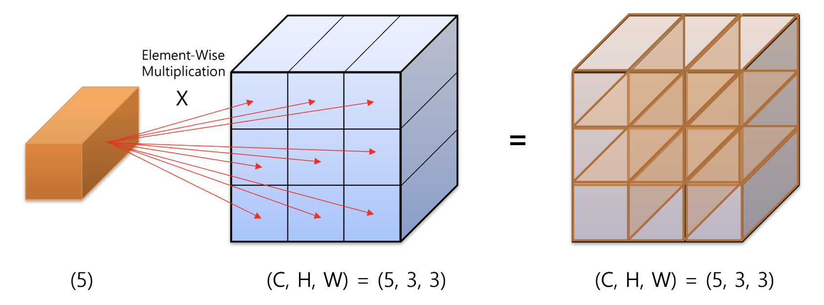
- 위 연산은 element 를 5 개 가지는 주황색의 vector 와
(C, H, W) = (5, 3, 3)을 element-wise multiplication 하는 연산이다. - multiplication 의 방향은
channel방향으로 곱해진다. 아래 코드를 보자.
T = torch.ones(5, 3, 3)
# tensor([[[1., 1., 1.],
#          [1., 1., 1.],
#          [1., 1., 1.]],

#         [[1., 1., 1.],
#          [1., 1., 1.],
#          [1., 1., 1.]],

#         [[1., 1., 1.],
#          [1., 1., 1.],
#          [1., 1., 1.]],

#         [[1., 1., 1.],
#          [1., 1., 1.],
#          [1., 1., 1.]],

#         [[1., 1., 1.],
#          [1., 1., 1.],
#          [1., 1., 1.]]])
V = torch.arange(1, 6) # tensor([1, 2, 3, 4, 5])
M은 파란색 tensor 로(5, 3, 3)크기에 1 로 이루어진 tensor 다. element-wise multiplication 되는 vectorV는 1 부터 5 까지를 element 로 가진다.- channel 방향으로 element-wise multiplication 을 하기 위해서 다음의 절차를 따른다.
- 먼저
view를 사용하여 vector 를 tensor 와 같은 shape 으로 맞추어 tensor 로 만든다. - 이후 두 tensor 를 곱한다.
- 먼저
T = torch.ones(5, 3, 3)
V = torch.arange(1, 6)
V_tensor = V.view(-1, 1, 1)

print(V_tensor, V_tensor.shape)
# tensor([[[1]],
#         [[2]],
#         [[3]],
#         [[4]],
#         [[5]]]) torch.Size([5, 1, 1])

element_wise_mul_result = V_tensor * T
print(element_wise_mul_result)
# tensor([[[1., 1., 1.],
#          [1., 1., 1.],
#          [1., 1., 1.]],

#         [[2., 2., 2.],
#          [2., 2., 2.],
#          [2., 2., 2.]],

#         [[3., 3., 3.],
#          [3., 3., 3.],
#          [3., 3., 3.]],

#         [[4., 4., 4.],
#          [4., 4., 4.],
#          [4., 4., 4.]],

#         [[5., 5., 5.],
#          [5., 5., 5.],
#          [5., 5., 5.]]])
Pytorch Setting
- Pytorch 를 사용할 때 일반적으로 import 하는 모듈과 GPU 관련 setting 이 있다.
- 먼저 아래는 기본적인 import 모듈들이다.
import torch
import torchvision
import torch.nn as nn # neural network 모음. (e.g. nn.Linear, nn.Conv2d, BatchNorm, Loss functions 등)
import torch.optim as optim # Optimization algorithm 모음 (e.g. SGD, Adam 등)
import torch.nn.functional as F # parameter 가 필요없는 Function 모음
from torch.utils.data import DataLoader # 데이터셋 관리 및 mini-batch 생성을 위한 함수 모음
import torchvision.datasets as datasets # 표준 데이터셋 모음
import torchvision.transforms as transforms # 데이터셋에 적용할 수 있는 변환 관련 함수 모음
import torch.backends.cudnn as cudnn # cudnn 을 다루기 위한 함수 모음

from torchsummary import summary # summary 를 통한 model 의 현황을 확인하기 위함
GPU Setting
- 아래는 딥러닝 학습에 필수적인 GPU 관련 Pytorch Setting 코드다.
torch.cuda.is_available() # cuda가 사용 가능한 지 확인

# cuda가 사용 가능하면 device에 "cuda" 를 저장하고 사용 가능하지 않으면 "cpu" 를 저장한다. Mac 용 GPU 인 "mps" 도 가능하다.
device = torch.device("cuda" if torch.cuda.is_available() else "cpu")
device = torch.device("mps" if torch.backends.mps.is_available() else "cpu")

# 멀티 GPU 사용. "0,1,2" 는 GPU 가 3 개 있고 그 번호가 0, 1, 2 인 상황
# 만약 GPU 가 5 개이고 사용 가능한 것이 0, 3, 4 라면 "0,3,4" 라고 적으면 된다.
os.environ["CUDA_VISIBLE_DEVICES"] = "0,1,2"

# 현재 사용가능한 GPU 사용 갯수 확인
torch.cuda.device_count()
torch.mps.device_count()

# 사용 가능한 device 갯수에 맞춰서 0 번 부터 GPU 할당
os.environ["CUDA_VISIBLE_DEVICES"] = ",".join(list(map(str, list(range(torch.cuda.device_count())))))

# cudnn 을 사용하도록 설정. GPU 를 사용하고 있으면 기본값은 True
import torch.backends.cudnn as cudnn
cudnn.enabled = True
- GPU device 의 사용 가능한 메모리를 코드 상에서 확인하려면 아래 함수를 사용한다.
# unit : byte
torch.cuda.get_device_properties("cuda:0").total_memory

# unit : mega byte
torch.cuda.get_device_properties("cuda:0").total_memory // 1e6

# unit : giga byte
torch.cuda.get_device_properties("cuda:0").total_memory // 1e9
- 멀티 GPU 사용 시 사용 시 아래 코드를 사용하여 전체 사용 가능한 GPU 메모리를 확인할 수 있다.
gpu_ids = list(map(str, list(range(torch.cuda.device_count()))))
total_gpu_memory = 0
for gpu_id in gpu_ids:
    total_gpu_memory += torch.cuda.get_device_properties("cuda:" + gpu_id).total_memory
GPU 메모리 해제 방법
- GPU 에 할당된 Tensor 를 GPU 에서 완전히 메모리 해제를 하려면 먼저 변수를 제거하고, cache 를 비워야 실제 메모리에서 해제된다.
- 변수가 제거되어도 cache 를 남겨두는 이유는 동일한 목적으로 변수가 생성될 때, 빠르게 생성하기 위하여 메모리를 잡고 있는 것이다. 왜냐하면 실제 Tensor 를 사용할 때, 반복적으로 Tensor 를 생성하기 때문이다.
- 만약 임시로 Tensor 를 만들었다가 제거해야 한다면 아래와 같이 변수 제거 후 cache 를 비우면 메모리에서 완전 제거된다.
- 변수 제거는
del 변수명을 사용하고 cache 를 비울 때에는torch.cuda.empty_cache()를 사용한다.torch.cuda.memory_allocated()는 tensor 가 현재 차지하고 있는 GPU 메모리를 bytes 단위로 출력한다.torch.cuda.memory_reserved()는 GPU 에서 cache 가 관리하는 메모리를 bytes 단위로 출력한다.
import torch

print(torch.cuda.memory_allocated()) # 0
print(torch.cuda.memory_reserved()) # 0

A = torch.rand(1000000000).cuda()
print(torch.cuda.memory_allocated()) # 4000000000
print(torch.cuda.memory_reserved()) # 4001366016

del A
print(torch.cuda.memory_allocated()) # 0
print(torch.cuda.memory_reserved()) # 4001366016

torch.cuda.empty_cache()
print(torch.cuda.memory_allocated()) # 0
print(torch.cuda.memory_reserved()) # 0
재현성을 위한 seed 값 고정
- 이전 포스트에서 다룬 내용이다.
- 같은 학습 데이터로 학습하고, 동일한 테스트 데이터로 테스트함에도 매번 실행해보면 모델의 학습 parameter 와 테스트 결과가 동일하지 않은 경우가 많다.
- 이는 높은 수준의 재생산성(Reproducibility)을 요구하는 대회나 업무에 지장을 줄 수 있다. 따라서 아래의 코드는 Pytorch 를 사용할 때 최대한 Reproducibility 를 유지할 수 있는 방법이다. 이를 통해 각 학습과 실험에서 디버깅과 재현을 유용하게 할 수 있다.
def seed(seed=42):
    random.seed(seed) # python random 모듈 seed 고정
    np.random.seed(seed) # numpy 의 seed 고정
    torch.manual_seed(seed) # pytorch 내부적으로 사용하는 seed 값 설정
    torch.cuda.manual_seed_all(seed) # if use multi-GPU
    torch.backends.cudnn.benchmark = False
    torch.backends.cudnn.deterministic = True
    torch.use_deterministic_algorithms(True) # Optional
    os.environ["PYTHONHASHSEED"] = str(seed)
댓글 남기기