[Deep Learning] MLP 구현 (3)

2024-10-29

MLP 를 사용하여 MNIST Classification 을 구현해보자.

필요 라이브러리

먼저 구현에 필요한 라이브러리를 import 해보자. Pytorch 를 사용할 것이고, GPU 대신 MPS 를 사용할 것이다.
또한 시각화를 위해 matplotlib 을 사용한다.

import numpy as np
import matplotlib.pyplot as plt
import torch
import torch.nn as nn
import torch.optim as optim
import torch.nn.functional as F

%matplotlib inline
%config InlineBackend.figure_format='retina'

plt.style.use('default')

print ("PyTorch version :[%s]."%(torch.__version__)) # PyTorch version: [2.5.0]

# cuda
device = torch.device('cuda:0' if torch.cuda.is_available() else 'cpu')

# mps
device = torch.device('mps' if torch.mps.is_available() else 'cpu')
print ("device: [%s]."%(device)) # device: [mps]

Dataset

MNIST 는 torchvision 에서 불러올 수 있는 간단한 이미지 데이터 세트로, 손으로 쓰여진 숫자 이미지들로 구성되어 있다.
숫자는 0 에서 9 까지로 모두 이미지 중심에 배치되어 있으며, 모든 이미지는 28 x 28 의 고정된 크기를 가진다.
torchvision.datasets 에서 사용할 수 있는 데이터셋은 공식문서에서 확인할 수 있다.
이렇게 공개된 데이터를 불러올 수도 있지만, 대부분의 프로젝트에서는 직접 데이터셋을 구현하고 custom Dataset 과 DataLoader 를 구현해야 한다.
- 이에 대한 구현과 연습은 해당 포스트에서 잘 정리했다.

from torchvision import datasets, transforms

mnist_train = datasets.MNIST(root='./data/',train=True, transform=transforms.ToTensor(),download=True)

mnist_test = datasets.MNIST(root='./data/',train=False,transform=transforms.ToTensor(),download=True)

print ("mnist_train: \n",mnist_train)
# mnist_train:
#  Dataset MNIST
#     Number of datapoints: 60000
#     Root location: ./data/
#     Split: Train
#     StandardTransform
# Transform: ToTensor() 

print ("mnist_test: \n",mnist_test)
# mnist_test:
#  Dataset MNIST
#     Number of datapoints: 10000
#     Root location: ./data/
#     Split: Test
#     StandardTransform
# Transform: ToTensor() 

위에서 보듯 train argument 를 통해 학습 데이터셋과 테스트 데이터셋을 구분해서 불러올 수 있다. 또한 transform 을 통해 이미지를 tensor 형태로 불러온다.
이렇게 불러온 데이터셋은 tuple 로 이루어져 있으며 각각 tensor 와 label 이다.

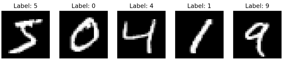
plt.figure(figsize=(10,10))

for idx in range(5):
    plt.subplot(1, 5, idx+1)
    
    # 시각화를 위해 (C x H x W) 에서 (H x W x C) 로 shape 변경 후 numpy 로 변환
    image = mnist_train[idx][0].permute(1, 2, 0).numpy()
    # 또는 아래의 방법도 가능
    image = mnist_train[idx][0].squeeze()

    plt.imshow(image, cmap='gray')
    plt.axis('off')
    plt.title("Label: %d"%(mnist_train[idx][1]))
    
plt.show() 

시각화 결과는 다음과 같다.

시각화 결과

Data Iterator

학습 과정에서 사용할 Data Iterator 를 정의한다. torch.utils.data.DataLoader 를 사용하며 batch_size 는 256 으로 한다.
또한 shuffle=True 를 주어 데이터가 고루 섞이게 하고, 해당 데이터를 불러오는 작업에 사용하는 서브 프로세스(subprocess) 개수를 나타내는 num_workers 를 1 로 한다.

BATCH_SIZE = 256

train_iter = torch.utils.data.DataLoader(mnist_train,batch_size=BATCH_SIZE,shuffle=True,num_workers=1)

test_iter = torch.utils.data.DataLoader(mnist_test,batch_size=BATCH_SIZE,shuffle=True,num_workers=1)

Define MLP

이제 MLP 를 구현해보자.
d2l 에서는 nn.LazyLinear 를 사용했지만, 여기서는 nn.Linear 를 사용하고 초기화를 모델 인스턴스화 시 실시하도록 한다.
유념해야 할 것은 여기서는 CNN 이 아닌 MLP 를 사용하기 때문에 이미지 데이터인 MNIST 데이터를 MLP 에 입력할 수 있게 바꿔줘야 한다.
MNIST 데이터 하나의 shape 은 (1, 28, 28) 이기 때문에 이를 (1, 784) 로 바꿔 모델에 입력시킨다.

class MLP(nn.Module):
    
    def __init__(self):
        super().__init__()
        self.in_dim = 784
        self.h_dim = 256
        self.out_dim = 10

        self.linear1 = nn.Linear(
            self.in_dim, self.h_dim
            )
        self.linear2 = nn.Linear(
            self.h_dim, self.out_dim
            )

        self.init_param()

    def init_param(self):
        for module in self.modules():
            
            if isinstance(module, nn.Linear):
                nn.init.kaiming_normal_(module.weight)
                if module.bias is not None:
                    nn.init.zeros_(module.bias)

    def forward(self, x):
        return self.linear2(F.relu(self.linear1(x)))

이후 이를 인스턴스화 하고 loss 와 optimizer 를 설정한다. Classification 이기 때문에 Cross Entropy loss 를 사용하고, optimizer 는 가장 많이 사용되는 Adam 을 사용한다.

mlp = MLP()
loss = nn.CrossEntropyLoss()
optimizer = optim.Adam(mlp.parameters(), lr=1e-3)

Forward Path

본격적으로 학습시키기 전에, 우선 모델의 forward path 를 점검해보자.
이 때 잊지 말아야 할 것은 입력 데이터와 모델의 parameter 가 같은 CPU 또는 GPU(MPS) 장치 위에 있어야 한다.

mlp.to(device)

x = torch.randn((2, 784), dtype=torch.float32, device=device)
y = mlp(x)

y_numpy = y.detach().cpu().numpy()
print(y)
# tensor([[ 1.2118,  1.9015,  1.1593,  1.5163, -1.5391,  1.6097, -1.2272, -1.2596,
#           5.1541, -0.6272],
#         [-0.7919, -1.6422,  1.6211,  0.4252, -0.0734,  0.7119, -3.1016, -1.4851,
#           4.0558,  0.5771]], device='mps:0', grad_fn=<LinearBackward0>)
print(y_numpy)
# [[ 1.2117767   1.9014747   1.159346    1.5163083  -1.5391197   1.609694
#   -1.2271589  -1.2595657   5.154105   -0.62723124]
#  [-0.7919306  -1.6421698   1.6211361   0.4252392  -0.07336473  0.7119251
#   -3.101596   -1.4850955   4.055849    0.5771163 ]]

위 결과를 보면 forward path 가 잘 작동하는 것을 확인할 수 있다.
위에서 torch.Tensor.detach().cpu().numpy() 를 해준 이유는 .detach() 를 통해 Autograd 의 computational graph 에서 해당 tensor 를 분리시키고, .cpu() 로 해당 tensor 를 CPU 메모리에 복사한 뒤 .numpy() 를 사용하여 numpy.ndarray 로 변경시켜 준 것이다.
이를 통해 output 시각화 등에 사용할 수 있다. 중요한 점은 GPU 와 CPU 사이의 transfer 는 속도가 느리기 때문에 지양해야 한다.
따라서 각각의 mini-batch 마다 해당 코드를 실행하는 것은 비효율적이고, 일정 epoch 마다 실행하거나 한 번에 CPU 로 옮기는 방식을 택하면 좋다.

Parameter Access

이제 MLP 의 parameter 를 보자. 아래 코드를 통하여 각 parameter 의 값과 MLP 가 가진 총 parameter 개수를 확인할 수 있다.

np.set_printoptions(precision=3) # 소수 셋째자리까지만 출력
n_param = 0 # 총 parameter 개수
for idx, (param_name, param) in enumerate(mlp.named_parameters()):
    param_numpy = param.detach().cpu().numpy()
    n_param += len(param_numpy.reshape(-1)) # parameter 개수 세기

    print ("[%d] param_name: [%s] shape: [%s]"%(idx, param_name, param_numpy.shape))
    print ("    val: %s"%(param_numpy.reshape(-1)[:5]))

# [0] param_name: [linear1.weight] shape: [(256, 784)]
#     val: [-0.02   0.042  0.01  -0.057 -0.011]
# [1] param_name: [linear1.bias] shape: [(256,)]
#     val: [0. 0. 0. 0. 0.]
# [2] param_name: [linear2.weight] shape: [(10, 256)]
#     val: [ 0.049  0.005 -0.12   0.115 -0.045]
# [3] param_name: [linear2.bias] shape: [(10,)]
#     val: [0. 0. 0. 0. 0.]

print ("Total number of parameters: [%s]"%(format(n_param,',d')))
# Total number of parameters: [203,530]

parameter initialization 이 잘 되었고, MLP 의 parameter 총 개수도 확인할 수 있다.

Evaluation

아직 학습시키지 않은 MLP 에 MNIST Classification 을 시키면 어떻게 나올까? Evaluation 코드를 구현하고 initial 성능을 확인해보자.
이 때 모델의 성능은 정확도(accuracy)를 통해 측정한다.

def eval(model, data_iter, device):
    with torch.no_grad():
        
        model.eval()

        n_total, n_correct = 0, 0
        for data, label in data_iter:
            target = label.to(device)
            model_pred = model(data.view(-1, 28*28).to(device))

            pred = torch.argmax(model_pred, dim=1)
            n_correct += (target == label).sum().item()
            n_total += data.size(0)

        val_acc = n_correct / n_total
        model.train()
    
    return val_acc

torch.no_grad() 는 해당 함수가 실행될 때는 학습할 때가 아니기 때문에 gradient 가 흐르지 않게 해준다.
또한 .eval() 을 사용한다. 여기서 구현한 MLP 에는 없지만 .eval() 을 사용하면 inference 단계에서 Dropout 이나 Batch Normalization 을 사용하지 않게 된다. 이후 .train() 을 사용하여 다시 모델이 학습할 때의 상태로 돌아간다.

mlp.init_param()
train_acc = eval(mlp, train_iter, device)
test_acc = eval(mlp, test_iter, device)

print ("train_acc: [%.3f], test_acc: [%.3f]"%(train_acc,test_acc))
# train_acc: [0.072], test_acc: [0.067]

위 결과를 보면 정확도가 10% 도 안될 정도로 매우 낮은 것을 확인할 수 있다.

Train

이제 학습 알고리즘을 구현해보자.

EPOCHS = 10

mlp.init_param()
mlp.train()

print("Start training")

for epoch in range(EPOCHS):
    sum_loss = 0
    for data, label in train_iter:

        pred = mlp(data.view(-1, 28*28).to(device))
        loss_out = loss(pred, label.to(device))

        # Update
        optimizer.zero_grad() # reset gradient
        loss_out.backward()   # back propagation
        optimizer.step()      # optimizer update

        sum_loss += loss_out

    avg_loss = sum_loss / len(train_iter)

    # print (inference)
    if epoch % 2 == 0:
        train_acc = eval(mlp, train_iter, device)
        test_acc = eval(mlp, test_iter, device)

        print ("epoch:[%d] loss:[%.3f] train_acc:[%.3f] test_acc:[%.3f]"%
               (epoch, avg_loss, train_acc, test_acc))

print("Complete training")

# Start training
# epoch:[0] loss:[0.379] train_acc:[0.945] test_acc:[0.943]
# epoch:[2] loss:[0.118] train_acc:[0.974] test_acc:[0.965]
# epoch:[4] loss:[0.071] train_acc:[0.984] test_acc:[0.973]
# epoch:[6] loss:[0.048] train_acc:[0.990] test_acc:[0.977]
# epoch:[8] loss:[0.033] train_acc:[0.992] test_acc:[0.977]
# Complete training

사실 위 구현에는 실제 딥러닝 프로젝트에서 구현할 학습 loop 에 비해 매우 간단한 상태다. 더구나 training 과 inference 가 같이 들어가 있다.
logging, early stopping, scheduler, checkpoint 등 굉장히 다양한 것이 있지만 여기서는 간단하게만 구현하였고 그 흐름만 보자.
또한 위에는 딥러닝 모델에서는 필수적인 validation 과정이 따로 들어가 있지 않다. 앞으로 작성하게 될 포스트에서는 CNN 이나 transformer 를 구현하면서 반드시 들어가야 할 것들을 포함한 학습 알고리즘을 구현할 것이다.
학습 결과, test 정확도가 97% 이상으로 잘 학습된 것을 볼 수 있다. 물론 over-fitting 이 발생한 것인지는 추후에 판단해봐야 한다.

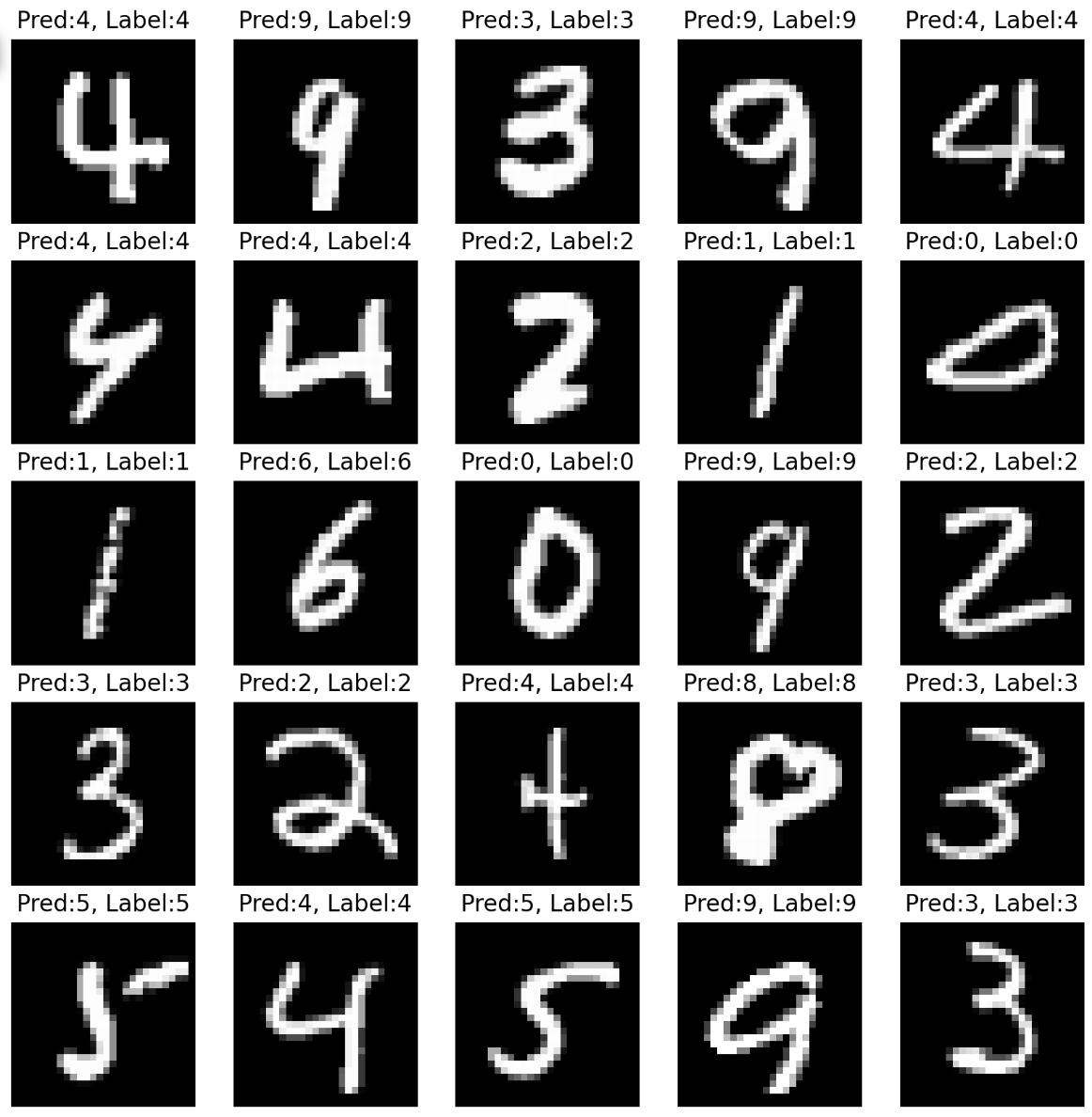
Test

이제 학습한 모델의 성능을 보자.
이 때 시각화를 위해 10000 개의 전체 테스트 데이터셋을 쓰기보다 25 개를 random 으로 뽑아서 진행한다.

n_sample = 25
sample_indices = np.random.choice(len(mnist_test.targets), n_sample, replace=False)
test_x = mnist_test.data[sample_indices]
test_y = mnist_test.targets[sample_indices]

with torch.no_grad():
    model_pred = mlp(test_x.view(-1, 28*28).type(torch.float32).to(device))

pred = model_pred.argmax(dim=1)

plt.figure(figsize=(10, 10))

for idx in range(n_sample):
    plt.subplot(5, 5, idx+1)
    plt.imshow(test_x[idx], cmap='gray')
    plt.axis('off')
    plt.title("Pred:%d, Label:%d"%(pred[idx],test_y[idx]))

plt.show()

아래 결과를 보면 굉장히 잘 분류해내는 것을 볼 수 있다.

시각화 결과

맨 위로 이동 ↑

Bkkhyunn

[Deep Learning] MLP 구현 (3)

필요 라이브러리

Dataset

Data Iterator

Define MLP

Forward Path

Parameter Access

Evaluation

Train

Test

댓글 남기기

관련 게시글

[Deep Learning, d2l] MLP 구현 (2)

[Deep Learning, d2l] MLP 구현 (1)

[Deep Learning, Optimization] Bias 와 Variance

[Segmentation] 8. Semantic Segmentation 연구 동향